The Maxima documentation says the numerical ODE solver in the command rk() is fourth order accurate. I ran a little test to confirm that.
Here’s the html export of the Maxima session, and a screenshot of the punchline:


The Maxima documentation says the numerical ODE solver in the command rk() is fourth order accurate. I ran a little test to confirm that.
Here’s the html export of the Maxima session, and a screenshot of the punchline:
I most often use the built-in solvers in MATLAB (or the freeware alternative FreeMat) for numerical solutions of ODE systems. They are easy to call and MATLAB graphical output is very flexible and of high quality. That said, if I’m already working in Maxima to study stability behavior and equilibrium solutions, it’s fun to stay in the same window for a numerical solution.
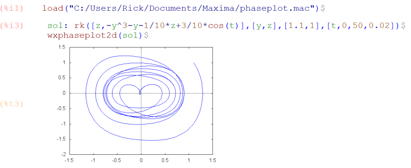
Here’s an example: a damped, driven hard spring oscillator, written in phase space variables
It’s straight-forward enough to run the Maxima numerical solver rk on this equation. Extracting the numerical values of the two dependent variables is a little bit of a drag, requiring a call to makelist. To make a plot in phase space, here’s a one-line function that is so easy to call:
/* wxphaseplot2d takes the output of s: rk([rhs1,rhs2])
   and  plots in phase space */
wxphaseplot2d(s):=wxplot2d([discrete,makelist([p[2],p[3]],p,s)],[xlabel,""],[ylabel,""]);
Here’s how it works on the above example with a cute phase-space solution curve:
And here’s another famous phase curve—the solution of the Brusselator:
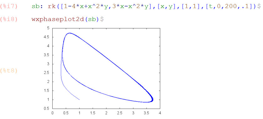
And can I just point out how analytically solving for the equilibrium solution has a very similar calling sequence — so easy that there’s no reason not to do it every time you want a numerical solution, and vice versa!

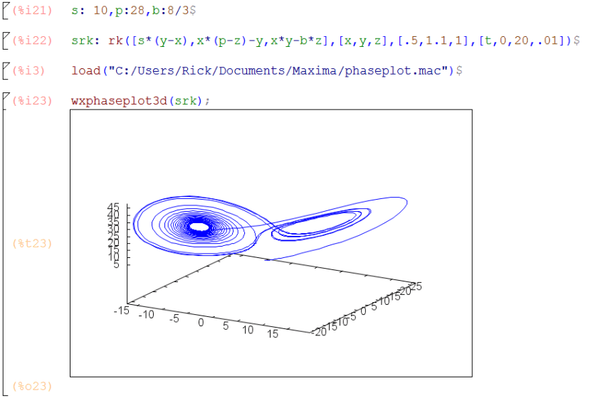
Update! Here’s a 3D phase plotter
/* wxphasplot3d takes the output of s: rk([rhs1,rhs2,rhs3]) and plots in phase space */
wxphaseplot3d(s):=wxdraw3d(point_type=0,point_size=.3,points_joined=true,points(makelist([p[2],p[3],p[4]],p,s)));
A classical example of 3D phase space trajectory curves, the Lorenz strange attractor system:
For my multivariable calculus class, I wanted an easy-to-call suite of symbolic integrators for path integrals of the form


My overarching design idea was that the input arguments needed to look the way they do when I teach the course:
 or a vector field
  or
or 
 defined by a vector-valued function
  where
where  as appropriate.
It took me a while to work out how to evaluate the integrand along the path within my function. Things that worked fine on the command line failed when embedded into a batch file to which I passed functions as arguments. I ended up using subst, one variable at a time. I’d like to be able to do this in a single command which can detect whether we’re in 2 or 3 dimensions so that I don’t need separate commands.
For now, here’s what I came up with along with some illustrative examples taken from Paul’s online math notes, that show how to call these new commands I, I2 and I3.
/* path integral of a scalar integrand f(x,y) on path r(t) in R^2, t from a to b */
 I(f,r,t,a,b):=block(
 [f1,f2,dr,Iout],
 f1:subst(x=r[1],f),
 f2:subst(y=r[2],f1),
 dr:sqrt(diff(r,t).diff(r,t)),
 Iout: integrate(f2*dr,t,a,b),
 Iout
 );
/* path integral of a vector integrand F(x,y) on path r(t) in R^2, t from a to b */ I2(H,r,t,a,b):=block( [H1,H2,I], H1:subst(x=r[1],H), H2:subst(y=r[2],H1), I: integrate( H2.diff(r,t),t,a,b), I );/* path integral of a vector integrand F(x,y,z) on path r(t) in R^3, t from a to b */ I3(H,r,t,a,b):=block( [H1,H2,H3,I], H1:subst(x=r[1],H), H2:subst(y=r[2],H1), H3:subst(z=r[3],H2), I: integrate( H3.diff(r,t),t,a,b), I );

Here’s an update: a related maxima function for evaluating a complex integral
where 


/* path integral of a complex integrand f(z): C --> C, on path z(t): R --> C, t from a to b */
IC(f,r,t,a,b):=block(
[f1,dz,Iout],
f1:subst(z=r,f),
dz:diff(r,t),
Iout: integrate(f1*dz,t,a,b),
Iout
);

I recently posted about : and := for defining functional expressions. I’m starting to enjoy these emoji-like constructions 😉
This is another colon-equals post. This time for defining functions involving the maxima differentiation command diff.
Notice below that if we define a function with :=, the naive use of :=diff doesn’t produce a derivative with the expected results upon evaluation.
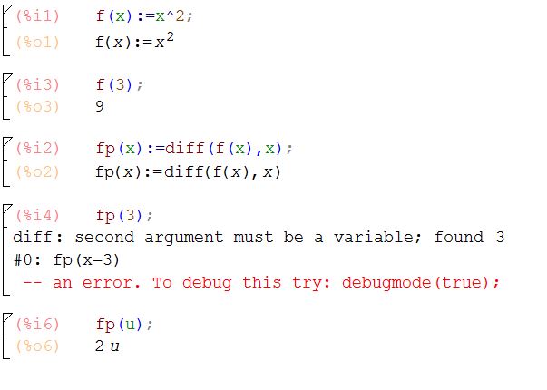
In fact, it’s a good thing that :=diff works like that. The error with fp(3) above comes from the fact that we’ve actually defined an operator that differentiates the function with respect to the argument we pass…in the case above, differentiating with respect to the symbol u makes sense, while differentiating with respect to the constant 3 doesn’t.
So how to make the derivative function do what we want? Two ways, that are subtly different, in ways I’m not completely sure of. More about that when I learn more :-).
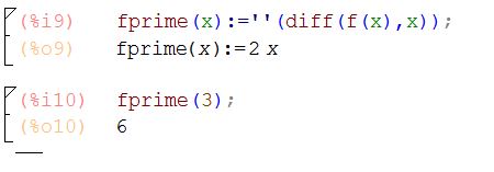
First is define,

Also you can use ”() quote-quote with parens around the whole right hand side:
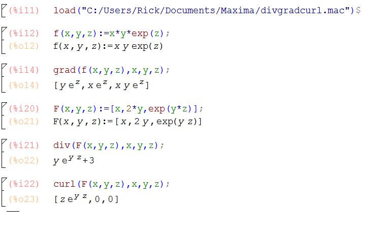
I used define to write functions for vector valued 3D curves in an earlier post. In figuring this out, I also learned that the :=diff form is really useful. Below are three little functions in which I use :=diff to define the vector calculus operators grad, div and curl. Notice that we pass the function f as an argument, and the :=diff form allows Maxima to differentiate them behind the scenes and return the results of the grad, div, and curl operators as you’d expect. These versions of div, grad and curl behave differently, and for me more as expected, than the functions of those names included in the Maxima vect package. You can download the .mac file here.
/* Three Maxima functions for the multivariable calculus operators grad, div, and curl
TheMaximaList.org, 2016
*/grad(f,x,y,z):=[diff(f,x),diff(f,y),diff(f,z)]$
div(f,x,y,z):=diff(f[1],x)+diff(f[2],y)+diff(f[3],z)$
curl(f,x,y,z):=[ diff(f[3],y)-diff(f[2],z),
diff(f[1],z)-diff(f[3],x),
diff(f[2],x)-diff(f[1],y) ]$
Here is a screenshot showing how to call these functions:
A classic topic in multivariable calculus involves the study of a vector valued function 


Here are maxima functions that compute these, called
unitT, unitN, unitB, and curvature. For a vector valued function 
T(t):=unitT(r(t),t);
You can download the .mac file here.
/* unitT computes the unit tangent vector for a vector valued function
of a scalar variable r(t)=[x(t),y(t),z(t)] */unitT(r,t):=
block([rp,rpn,T],
define(rp(t),diff(r,t)),
define(rpn(t),sqrt(rp(t).rp(t))),
define(T(t),rp(t)/rpn(t)),
trigsimp(T(t))
)$/* unitN computes the unit normal vector for a vector valued function
of a scalar variable r(t)=[x(t),y(t),z(t)]
unitN requires unitT */unitN(r,t):=
block([T,Tp,Tpn,N],
define(T(t),unitT(r,t)),
define(Tp(t),diff(T(t),t)),
define(Tpn(t),sqrt(Tp(t).Tp(t))),
define(N(t),Tp(t)/Tpn(t)),
trigsimp(N(t))
)$/* unitB computes the unit normal vector for a vector valued function
of a scalar variable r(t)=[x(t),y(t),z(t)]
unitB requires unitT and unitN */unitB(r,t):=
block([T,N,B],
define(T(t),unitT(r,t)),
define(N(t),unitN(r,t)),
define(B(t),[T(t)[2]*N(t)[3]-T(t)[3]*N(t)[2],
T(t)[3]*N(t)[1]-T(t)[1]*N(t)[3],
T(t)[1]*N(t)[2]-T(t)[2]*N(t)[1]]),
trigsimp(B(t))
)$/* curvature computes the curvature
curvature requires unitT */curvature(r,t):=
block([T,Tdot,rdot,K],
define(T(t),unitT(r,t)),
define(Tdot(t),diff(T(t),t)),
define(rdot(t),diff(r,t)),
define(K(t),trigsimp(sqrt(Tdot(t).Tdot(t)/rdot(t).rdot(t)))),
K(t)
)$


