A Package of Maxima Utilities for my Ordinary Differential Equations Course: MATH280.mac


I’ve put together a collection of functions — some direct quotes of other contributed functions, some renamed or repackaged, and some newly implemented — for various needed tasks in my undergraduate ordinary differential equations course.

I’ve written elsewhere about the Backward Difference Formula implementations, the phase space visualization functions,  the matrix extractors, and  the numerical solutions plotters.

The package includes my home-grown help utility.

You can download the package MATH280.mac

…and if you’re interested, here’s my multivariable calculus package MATH214.mac

MATH280.mac contains:
 wxphaseplot2d(s)
 wxphaseplot3d(s)
 phaseplot3d(s)
 wxtimeplot(s)
 plotdf(rhs)
 wxdrawdf(rhs)
 sol_points(numsol,nth,mth)
 rkf45(oderhs,yvar,y0,t_interval)
 BDF2(oderhs,yvar,y0,t_interval)
 BDF2a(oderhs,yvar,y0,t_interval)
 odesolve(eqn,depvar,indvar)
 ic1(sol,xeqn,yeqn)
 ic2(sol,xeqn,yeqn,dyeqn)
 eigU(z)
 eigdiag(z)
 clear()
 -
 -
 for any of the above functions,
 help(function_name) returns help lines for function_name
 -
 Last Modified 5:00 PM 3/27/2017

Plotting Numerical Solutions of Ordinary Differential Equations in Maxima

Maxima comes with a few well-implemented numerical ODE solvers — rk() and rkf45() — and I’ve written in a previous post about my variable stepsize implementation of the 2nd order backward differentiaion formula for stiff systems  BDF2a().

Plotting the resulting numerical solutions — which is a list of lists of the form

[[indvar, depvar1, depvar2,… ], [indvar, depvar1, depvar2,… ], …   ]

with each of the sublists  representing the state of the system at a discrete time — requires a little familiarity with list functions like makelist() and map().

Here are a few little helper routines to make that quicker:

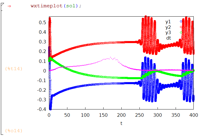
wxtimeplot()

This is mainly a teaching tool for my ordinary differential equations course, taking the output of the solver and, assuming there aren’t more than three dependent variables, plotting all the dependent variables vs the independent variable on the same set of axes, with a representation of the step size.
wxtimeplot

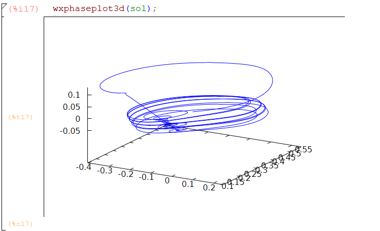
wxphaseplot2d,wxphaseplot3d

I wrote about these in another post
wxphaseplot3d

sol_points()

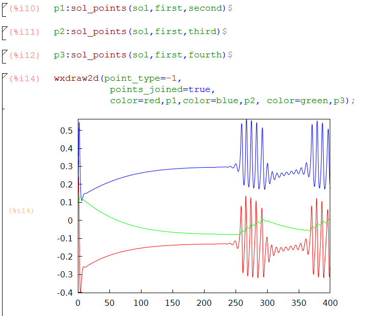
This is a more general purpose function.  Given the output of the numerical ode solver, this constructs a points() subcommand ready to plug into draw2d().  This allows for the full generality of draw2d:  colors, axis labels, point points,

Especially useful for plotting results from more than one call to the solver, such as when we need to see the effect of changing a parameter value:
sol_points

Below I’ve pasted the code for the plots, and also for the interesting differential equations from  Larter et al in Chaos, V.9 n.3 (1999)

(tw:(cosh((Vi-V3)/(2*V4))^(-1)),
m:(1/2)*(1+tanh((Vi-V1)/V2)),
w:(1/2)*(1+tanh((Vi-V3)/V4)),
aexe:aexe1*(1+tanh(Vi-V5)/V6),
ainh:ainh1*(1+tanh((Zi-V7)/V6))
)$

(rhs1:-gCa*m*(Vi-1)-gK*Wi*(Vi-ViK)-gL*(Vi-VL)+I-ainh*Zi,
 rhs2:(phi*(w-Wi)/tw),
 rhs3:b*(c*I+aexe*Vi)
 )$ 

(V1:-.01,V2:0.15,V3:0,V4:.3,V5:0,V6:.6,V7:0,
 gCa:1.1,gK:2,gL:0.5,VL:-.5,ViK:-.783,phi:.7,tw:1,
 b:0.0809,c:0.22,I:0.316,aexe1:0.6899,ainh1:0.695)$

 load(rkf45);

 sol:rkf45([''rhs1,''rhs2,''rhs3],[Vi,Wi,Zi],[.1,.1,.1],[t,0,400],
             report=true,absolute_tolerance=1e-8)$
sol_points(numsol,nth,mth):=points(map(nth,numsol),map(mth,numsol));
/* wxtimeplot takes the output of sol: rk45 and plots 
 up to 3 dependent variables 
plus the scaled integration step size vs time*/
wxtimeplot(sol):=block(
[t0,t,tt,dt,big,dtbig],
t0:map(first,sol),
t:part(t0,allbut(1)),
tt:part(t0,allbut(length(t0))),
dt:t-tt,
dtbig:lmax(dt),
big:lmax(map(second,abs(sol))),
if is(equal(length(part(sol,1)),3)) then(
 big: max(big,lmax(map(third,abs(sol)))),
 wxdraw2d(point_type=6, key="y1",
 points(makelist([p[1],p[2]],p,sol)),
 color=red, key="y2",
 points(makelist([p[1],p[3]],p,sol)),
 color=magenta, key="dt",point_size=.2,
 points(t,big*dt/dtbig/4),xlabel="t",ylabel=""))
elseif is(equal(length(part(sol,1)),2)) then
 wxdraw2d(point_type=6, key="y1",
 points(makelist([p[1],p[2]],p,sol)),
 color=magenta, key="dt",point_size=.2,
 points(t,big*dt/dtbig/4),xlabel="t",ylabel="")
elseif is(equal(length(part(sol,1)),4)) then(
 big: max(big,lmax(map(third,abs(sol)))),
 big: max(big,lmax(map(fourth,abs(sol)))),
 wxdraw2d(point_type=6, key="y1",
 points(makelist([p[1],p[2]],p,sol)),
 color=red, key="y2",
 points(makelist([p[1],p[3]],p,sol)),
 color=green, key="y3",
 points(makelist([p[1],p[4]],p,sol)),
 color=magenta, key="dt",point_size=.2,
 points(t,big*dt/dtbig/4),xlabel="t",ylabel=""))
 );

Jordan Canonical Form in Maxima

After not easily finding such a thing from a cursory search of the Maxima documentation, I spent a few hours over the weekend beginning to write a Maxima function to compute, for any given square matrix M , an invertible matrix P so that

P^{-1}MP = J

where J is the Jordan matrix that displays the eigenvalue/vector structure of M.

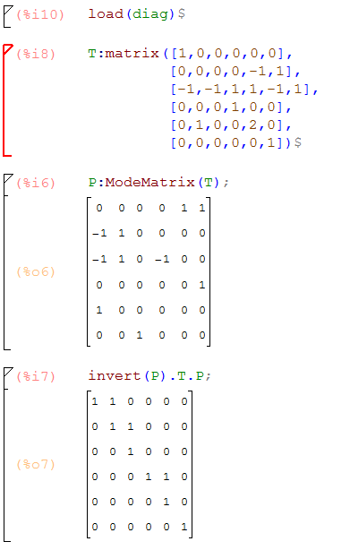
It took several searches for me to find, but of course there’s already such a  function — with a not so easily searched-for name — in the diag package:   ModeMatrix()


ModeMatrix

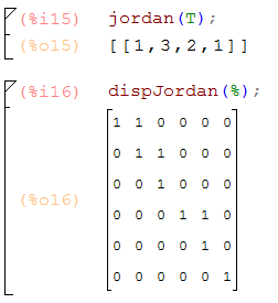
To see just the matrix J, diag provides jordan() and dispJordan()

dispJordan

How to fix the \tag{}\label{} glitch in the wxMaxima “export to HTML” output

wxmaxima_tag_error

**Update:   This seems to be fixed in  wxMaxima versions > 16.04, but it remains an issue for MacOS users, who for the moment are stuck with an older version of wxMaxima.*****

The work flow in some of my classes involves:

  1. students doing work in wxMaxima
  2. exporting to HTML
  3. printing as PDF
  4. submitting the resulting document to a Dropbox link

The process is usually very slick, with only a few headaches.  Here is one such pain:  occasionally the result of a Maxima command will be displayed in the HTML document like as

wxmaxima_tag_error

That seems to happen if the expression name (here the matrix A) has been used before in the same session and the mathjax  latex-ish tag labeling gets confused by a multiply-defined tag.

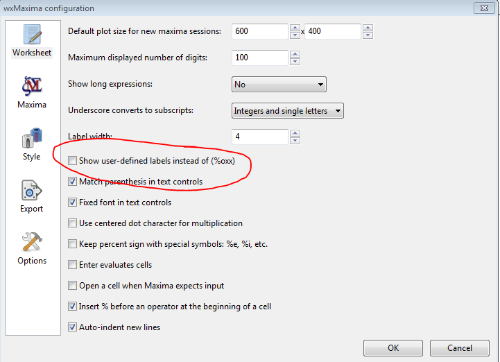
To work around that, unselect the “Show user-defined labels instead of (%oxx)” option in Configure/Preferences.  That way, unless an exported document is the result non-re-evaluated cells between several Maxima sessions, the labels should be unique.

tag_error_fix

And one last thing:  If the work has been done (and saved) between several wxMaxima seesions, it’s possible that the number output lines like %o23 etc  might not be unique, so before exporting, I suggest Cell –> Evaluate All Cells.

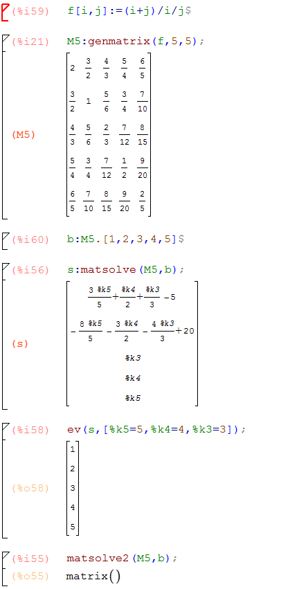
Solve Ax=b in Maxima, part 2

In a previous post, I included my little coding project to implement a general backsolve() function to use with the built-in maxima matrix function echelon(), producing an easy-to-call matrix solver matsolve(A,b).  The result is meant to solve a general matrix vector equation Ax=b , including cases when A is non-square and/or non-invertible.

Here’s a quicker approach — convert the matrix into an explicit system of equations using a vector of dummy variables, feed the result into the built-in Maxima function linsolve(), and then extract the right hand sides of the resulting solutions and put them into a column vector.

The two methods often behave identically, but here’s an example that breaks the linsolve() method, where the backsolve() method gives a correct solution:

matsolve2breaks


*Note, I’ve found that the symbol rhs is a very popular thing for users to call their problem-specific vectors or functions.  Maxima’s  “all symbols are global” bug/feature generally wouldn’t cause a problem with a function call to rhs(), but the function map(rhs, list of equations)  ignores that rhs() is a function and uses user-defined rhs.  For that reason I protect that name in the block declarations so that rhs() works as expected in the map() line at the bottom.  I think I could have done the same thing with a quote: map(‘rhs, list of equations).

matsolve2(A,b):=block(
 [rhs,inp,sol,Ax,m,n,vars],
 [m,n]:[length(A),length(transpose(A))],
 vars:makelist(xx[i],i,1,n,1),
 Ax:A.vars,
 inp:makelist(part(Ax,i,1)=b[i],i,1,n,1),
 sol:linsolve(inp,vars),
 expand(transpose(matrix(map(rhs,sol))))
);