logarc
In the back of my calculus book there is a table of famous integrals. Here’s integral number 21 in that table:

From Maxima integrate(), I get

What’s going on?
Both forms give a workable antiderivative for the original integrand:

Furthermore, we believe that both forms are correct because of this helpful identity for hyperbolic sine:

Turns out (thanks to a Barton Willis for pointing me in the right direction) there’s a variable logarc that we can set to make Maxima return the logarithmic form instead of hyperbolic sine:

I haven’t yet encountered cases where this would be a bad idea in general, but I’ll update this if I do.
logabs
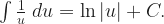
In the first week of my differential equations course, we study methods of direct integration and separation of variables. I like to emphasize that the absolute values can lend an extra degree of generality to solutions with antiderivatives of the form
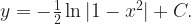
As an example, for the initial value problem


it is convenient for treating all possible initial conditions (
However, Maxima omits the absolute values.

For this case, we could consider only the needed interval 
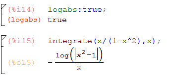
Turns out we can set the Maxima variable logabs to make integrate() include absolute values in cases like this:
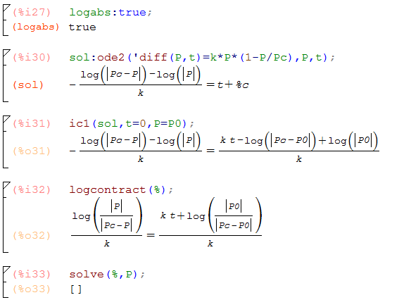
But then later in the course, I saw that logabs also impacts the Ordinary Differential Equation solver ode2(). I encountered an example for which Maxima, in particular solve() applied to expressions involving absolute value, didn’t do what I wanted with logabs:true
For the logistic equation
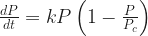

we expect that by separating variables we can obtain the solution

Here’s what happens when we use ode2() with and without logabs:true:

 ,
, , or
, or .
. or a vector field
 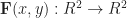 or
or 
 defined by a vector-valued function
  where
where  as appropriate.

 and the curve
  is given by
  .
.