

In response to several nearly simultaneous queries, I’ve been working this week on generating a 3D plot and creating a mesh file from within Maxima that is suitable for exporting to a 3D printer.
As a guide, I used this 2012 article from the Mathematical Intelligencer by Henry Segerman. The idea is to draw a surface using traces made from parametric tubes, then export that to a .PLY format file.
Here’s my prototype for the process of generating the surface, reading in the resulting gnuplot data file, identifying faces appropriately, and writing into a .PLY file.
That isn’t yet ready for the 3D printer, but I could load it into the free program MeshLab, and from there convert to .STL
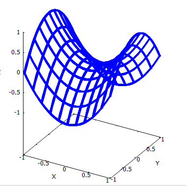
Here’s my figure from Maxima:
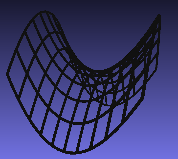
And the resulting .PLY file loaded into MeshLab
Here’s a few seconds of video from the printing process
And 2.5 hours later, the low resolution first-try 3D printed object:

 . Notice for the smallest radius pre-image, the image under
  is largely unchanged. As radius grows the image forms a loop then doubles on itself. Here’s a fun insight: that looping behavior occurs at radius .75, a circle containing a point
  at which
  . More on this later, but its exciting to find a geometric significance of a zero of the derivative, considering how much importance such points have in real calculus. Finally the third figure shows really interesting behavior for the function
  . Notice again the looping brought about by points at which the derivative is zero. Notice also the change in direction of the image each time we cross over a pole—that is a root of the denominator. The maxima code is given below.


