Eulix: A Stiff ODE Solver in Maxima

Look what I found in the share/contrib directory:

There isn’t any documentation available from texinfo:

Browsing around on the web I found this documentation page.

There are also many examples given in the Eulix_*.mac files in share/contrib/Eulix . Here’s what is says at the top of Eulix.mac:

* (C) Helmut Jarausch
 *
 * @version 1.0 Date August 29th, 2017
 *
 * @author Helmut Jarausch
 *         RWTH Aachen University

 * @contents
 *  Eulix is an linearly implicit (by default) extrapolated Euler method.
 *  It uses variable step sizes, variable orders and offers dense output.
 *  Eulix can solve systems like  M y'(t)= f(t,y)  where M is a constant mass
 *  matrix. This enables the solution of differential algebraic equations (DAE)
 *  of index 1, as well.
 *
 *  I have made a simplified version of  SEULEX  published in
 *
 *  E. Hairer, G.Wanner
 *  Solving Ordinary Differential Equations II
 *  Stiff and Differential-Algebraic Problems
 *  Springer 1991

A Test Problem: The Ball of Flame

To test drive the method, I’ll retrace Cleve Moler’s steps in this excellent piece about numerical solvers for stiff equations.

We’ll consider the “ball of flame” equation of Lawrence Shampine:

\dot{y}=y^2-y^3, \;\;\;\;\;\;  y(0)=\delta

on the time interval 0 \le t \le 2/\delta     .

The equation is meant to be a simple model of flame propagation, but it could also describe what happens to non-stiff solvers for small values of \delta    : they go down in a ball of flames!

Notice that the basic calling sequence for Eulix() is the same as for rkf45(). The first thing to observe is that when applied to the ball of flame, Eulix() uses less time and less steps than rkf45():
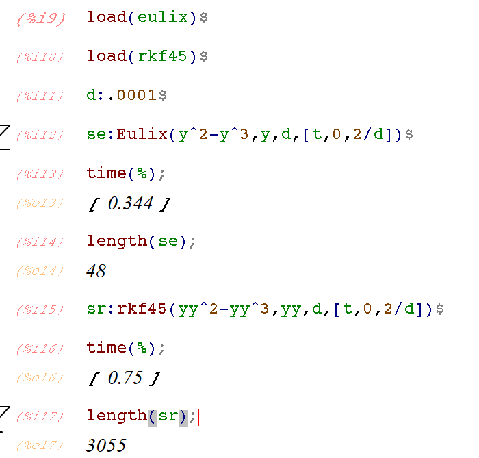
Plots of the solution points show that Eulix() makes this look like an easy problem, using very few points for the horizontal parts of the solution, and concentrating more points at the sharp turns:

The non-stiff variable step Runge-Kutta-Fehlberg method rkf45() makes this look hard:
Zooming in shows how hard rfk45() is working on the horizontal part of the solution. It is doing its job to maintain the error within the default tolerance 1e-6, but it’s using a lot of steps and function evaluations to do that:

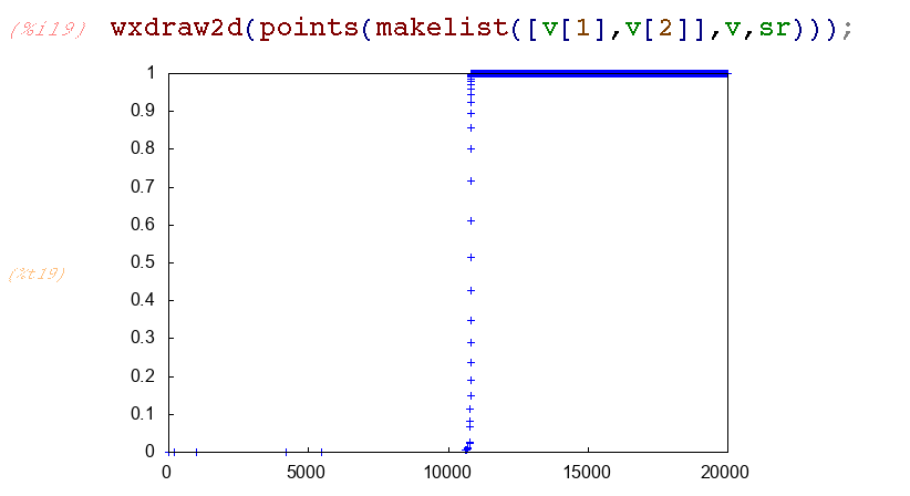
And one final thing to know about Eulix(): The output can appear very sparse, as we see in the region t> 10000 in the figure above. There’s an easy option to specify dense output (likely computed using splines and the existing solution points). Add the desired output interval as a fourth entry in the time specification list: [t,tstart,tfinal,output_interval]

Thank you Helmut Jarausch!

Advertisement

Quotes, global variables, and ODE solvers.

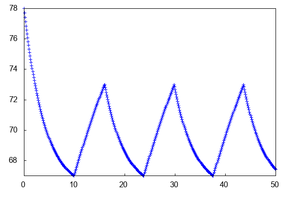
Computed solution: room temperature in a model of a thermostatically switched air conditioning system

Every winter term in my introductory ordinary differential equations class, I ask each of my students to choose from the scientific literature a paper that puts ODE models at the center of the work, and to reproduce the author’s results. For the past 5 years we’ve used Maxima for that purpose, and throughout the course for both symbolic and numerical tasks.

A perennial favorite is “Temperature Models for Ware Hall” by J. K. Denny and C. A. Yackel, The College Mathematics Journal, Vol. 35, No. 3 (May, 2004), pp. 162-170 http://www.jstor.org/stable/4146891 .

We have a first order ODE that combines two Newton’s law of cooling processes: the room is in thermal contact with the hot outside air at 90F and with cooled air at 60F coming from the air conditioner.

\frac{dT}{dt}=0.2(90-T)+0.2S(T)(60-T)

The idea is to model an air conditioning system that is controlled by a thermostatic switch. In the model above the switch function S(T)=1 when the cooling sytem is running, becomes zero if the system is running and the temperature reaches 67F, becomes 1 if the system is not running and the temperature reaches 73F. The behavior of the room temperature is shown in the figure at the top of this piece.

There might be another way to model this (I’d be delighted to learn what that is!) but here we treat the thermostat with a global variable that can be read and changed within a numerical solver as part of the right-hand-side function.

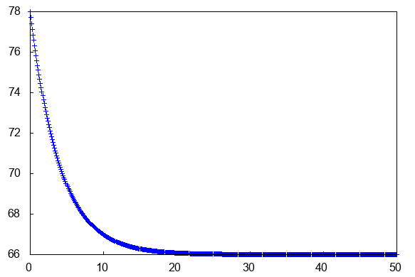
The question in this post is: how to implement a global flag like that in Maxima? Below are four variants involving various combinations of the Maxima quote operator. The first two give the hoped-for behavior and were used to produce the figure above. The last two don’t seem to have access to the global flag and the cooling system runs without ceasing. I include a graph of that incorrect computed solution at the bottom of this post.

The Details

  • In the first case, the switch function is included in the right-hand-side function with a single quote.
  • In the second, the switch in included with quote-quote, but the order in which the right hand side and switch is important: the switch function must be defined AFTER the right hand side function in which it is called
  • In the third, the switch in included with quote-quote, but the order from above is reversed and the global flag seems undetected.
  • In the fourth, the switch is included without quote or quote-quote and the behavior is same as quote-quote in the second and third cases.

I don’t know why each works or doesn’t! I’m hoping you do and can tell me 🙂 Thanks in advance.

/*This works as intended with single-quote on ThermSwitch
    ThermSwitch can be defined either before or after ff */
kill(all);
globalAC:1;

ThermSwitch(T):=block(
	      if T<67 then globalAC:0
	         else if T>73 then globalAC:1,
	      return(globalAC))$
		  
ff:.05*(90-T) + .2*'ThermSwitch(T)*(60-T);

s:rk(ff,T,78,[t,0,50,.1])$
wxdraw2d(points(makelist([p[1],p[2]],p,s)));
/*This works as intended with double-quote on ThermSwitch
    ThermSwitch  defined  AFTER ff */
kill(all);
globalAC:1;

ff:.05*(90-T) + .2*''ThermSwitch(T)*(60-T);

ThermSwitch(T):=block(
	      if T<67 then globalAC:0
	         else if T>73 then globalAC:1,
	      return(globalAC))$
		  
s:rk(ff,T,78,[t,0,50,.1])$
wxdraw2d(points(makelist([p[1],p[2]],p,s)));
/*This does NOT work as intended with double-quote on ThermSwitch
    ThermSwitch  defined  BEFORE ff */
kill(all);
globalAC:1;

ThermSwitch(T):=block(
	      if T<67 then globalAC:0
	         else if T>73 then globalAC:1,
	      return(globalAC))$
		  
ff:.05*(90-T) + .2*''ThermSwitch(T)*(60-T);

s:rk(ff,T,78,[t,0,50,.1])$
wxdraw2d(points(makelist([p[1],p[2]],p,s)));
/*This does NOT work as intended with unquoted ThermSwitch before ff
   it does work as intended with unquoted ThermSwitch after ff  */
kill(all);
globalAC:1;

ThermSwitch(T):=block(
	      if T<67 then globalAC:0
	         else if T>73 then globalAC:1,
	      return(globalAC))$
		  
ff:.05*(90-T) + .2*ThermSwitch(T)*(60-T);

s:rk(ff,T,78,[t,0,50,.1])$
wxdraw2d(points(makelist([p[1],p[2]],p,s)));
Incorrect Computed solution: room temperature in a model of a thermostatically switched air conditioning system — the thermostatic switch in the model isn’t functioning correctly.

Collecting all my little matlab-like Maxima widgets in one place

Since I’ve been using Maxima (circa 2016), I’ve occasionally missed some little feature from matlab and coded up a replacement for maxima, with a corresponding blog piece here at the Maximalist.

Some examples are find(), diff(), pause(), size(), cumsum(), diag(), and a few list indexing utilities. Also a help() utility that mimics matlab.

Here’s a mac file with all of those in one easy-to-load place: matlabesque.mac

Its help() entry reads like this:

matlabesque.mac contains:
 find(exp)
 ithruj(L,i,j)
 indexby(L,indexlist)
 matlab_diff(L)
 pause([options])
 cumsum(l)
 size(M)
 diag(M)
 -
 -
 for any of the above functions,
 help(function_name) returns help lines for function_name