Surface Integrals, Triple Integrals, and the Divergence Theorem of Gauss in Maxima

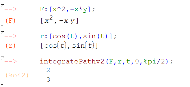
In earlier posts, I describe the Package of Maxima functions MATH214 for use in my multivariable calculus class, with applications to Greens  Theorem and Stokes Theorem.

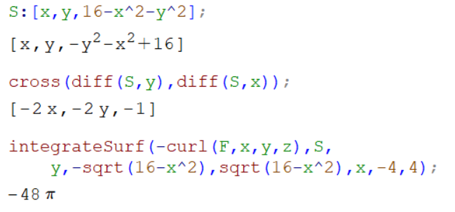
Here we show how the  surface integral function integrateSurf() and triple integration  function integrate3()  (together with the divergence function div() )work on a Gauss’s Theorem example:

Gauss2

We integrate the parabolic surface and the circular base surface separately, and show their sum is equal to the triple integral of the divergence.

Gauss1

The functions above are included in the MATH214 package, but I list them below as well:

integrateSurf(F,S,uu,aa,bb,vv,cc,dd):=block(
 [F2],
 F2:psubst([x=S[1],y=S[2],z=S[3]],F),
 integrate(integrate(trigsimp(F2.cross(diff(S,uu),diff(S,vv))),uu,aa,bb),vv,cc,dd));

integrate3(F,xx,aa,bb,yy,cc,dd,zz,ee,ff):=block(
 integrate(integrate(integrate(F,xx,aa,bb),yy,cc,dd),zz,ee,ff));

div(f,x,y,z):=diff(f[1],x)+diff(f[2],y)+diff(f[3],z)$

cross(_u,_v):=[_u[2]*_v[3]-_u[3]*_v[2],_u[3]*_v[1]-_u[1]*_v[3],_u[1]*_v[2]-_u[2]*_v[1]]$


Path Integrals in the Plane, Double Integrals, and Greens Theorem in Maxima

In an earlier post I described the Maxima package MATH214 for use in my multivariable calculus class.  I’ve posted examples with applications to Gauss’s  Theorem and Stokes Theorem.

Here we take the double integration routine integrate2() and the 2D path integral integratePathv2() for a spin with a Green’s Theorem example from Stewart’s Calculus Concepts and Contexts:

Greens2

Greens1

And of course polar coordinates are nice too:

Greens3.PNG

The two functions used above are included in the MATH214 package, but I list them below as well.

integratePathv2(H,r,t,a,b):=block(
[H2],
H2:psubst([x=r[1],y=r[2]],H),
 integrate( trigsimp(H2.diff(r,t)),t,a,b)
);

integrate2(F,xx,aa,bb,yy,cc,dd):=block(
 integrate(integrate(F,xx,aa,bb),yy,cc,dd));


Surface Integrals and Stokes Theorem in Maxima


In an earlier post I detailed the Maxima functions contained  the MATH214 package for use in my multivariable calculus class.  The package at that link has now been updated with some further integration utilities:  integrate2() and integrate3() for double and triple integrals and integrateSurf() for surface integrals of vector fields in 3D.  I’ve posted examples with applications to Green’s  Theorem and Gauss’s Theorem.

Here’s a test drive of the surface integration function using a Stokes theorem example I found on the web:

Verify Stokes theorem for the surface S described by the paraboloid z=16-x^2-y^2 for z>=0

and the vector field

F =3yi+4zj-6xk

First the path integral of the vector field around the circular boundary of the surface using integratePathv3() from the MATH214 package

Stokes1

And also the surface integral using integrateSurf().  Notice that in the order of integration we specify in integrateSurf(),  (first  y then x) the surface normal vector computed with cross() in that same variable order points inward—the negative orientation.  We reverse the direction with an extra negative inside the surface integral.

Stokes2

Although they are included in the MATH214 package, here are the  functions used above:

integrateSurf(F,S,uu,aa,bb,vv,cc,dd):=block(
 [F2],
 F2:psubst([x=S[1],y=S[2],z=S[3]],F),
 integrate(integrate(trigsimp(F2.cross(diff(S,uu),diff(S,vv))),uu,aa,bb),vv,cc,dd));

cross(_u,_v):=[_u[2]*_v[3]-_u[3]*_v[2],_u[3]*_v[1]-_u[1]*_v[3],_u[1]*_v[2]-_u[2]*_v[1]]$

curl(f,x,y,z):=[ diff(f[3],y)-diff(f[2],z),curl(f,x,y,z):=[ diff(f[3],y)-diff(f[2],z),                     diff(f[1],z)-diff(f[3],x),   diff(f[2],x)-diff(f[1],y) ]$
integratePathv3(H,r,t,a,b):=block(
[H3],
H3:psubst([x=r[1],y=r[2],z=r[3]],H),
 integrate( trigsimp(H3.diff(r,t)),t,a,b)
);


An undocumented synonym for diff() in Maxima

Today, a student turned in some Maxima work for my class. I discovered he had successfully used the command derivative() in place of diff() with seemingly identical results.  I verified that the same thing works in several versions of Maxima I have installed on my windows computer.  Who knew?

diffderivative

Multiple plots in a single Maxima figure

In MATLAB, I often use the subplot() command to make an array of multiple plots in a single figure.

In Maxima, we can achieve that by generating each of the subplots using gr2d(),  and then putting them all together with a call to draw() or wxdraw():

2scenes

There’s an optional columns argument — the subplots are drawn row-wise in an array with the specified number of columns:

3scenes

And of course all this works for 3d plots using gr3d():

3dscenes

3D Printing and Maxima

In response to several nearly simultaneous queries, I’ve been working this week on generating a 3D  plot  and creating a mesh file from within Maxima  that is suitable for exporting to a 3D printer.

As a guide, I used this 2012 article from the Mathematical Intelligencer by Henry Segerman.  The idea is to draw a surface using traces made from parametric tubes, then export that to a .PLY format file.

Here’s my prototype for the process of generating the surface, reading in the resulting gnuplot data file, identifying faces appropriately, and writing into a .PLY file.

That isn’t yet ready for the 3D printer, but I could load it into the free program MeshLab, and from there convert to .STL

Here’s my figure from Maxima:

pringle

And the resulting .PLY file loaded into MeshLab


saddle_meshdraw

Here’s a few seconds of video from the printing process

And 2.5 hours later, the low resolution first-try 3D printed object:

3dprintverision01

Computing and Visualizing Path Integrals of Vector Fields

A few months ago, I posted my path integral functions, which are included in the MATH214 package.  Recently, I came across something I’d been looking for:  a Maxima utility for visualizing vector fields.  Its in the Maxima/Share directory under drawutils.

Written in 2010 by Donald J Bindner, the commands plot_vector_field and plot_vector_field3d do almost everything I was looking for.  The drawback is that I wanted to plot the vector fields along with the integration path.  I modified those two commands slightly into versions called make_vector_field  and make_vector_field3d to produce the lists of vectors for plugging into draw2d and draw3d, so that I could include the vector fields in  bigger graphics calls.  My modifications are available here.  The package includes my home-baked help utility.

Here’s what the path integral command and the vector field generator look like on an example from chapter 13 of Stewart’s “Calculus Concepts and Contexts”

StewartPathIntegralExample

StewartVectorFieldIntegralPicture

Solvers!

A few months ago, when I was very new to Maxima, I posted my solutions to several multivariable optimization problems, and included a standard constrained optimization example for which the built in command solve failed.

Here’s the problem:

MinVolConstArea

In my multivariable calculus class, we’ve just encountered that problem again.  What my students and I discovered was that the order of the variables as specified by the user in the argument list caused the command to either succeed or fail, as you can see from the first two lines below:

Ksolve

I wrote to the experts at maxima-discuss@lists.sourceforge.net.  They replied en masse very quickly and were very generous with their time and advice. They verified the problem, pointing out that solving systems of equations is really complicated, and that the solve program seeks to solve for the variables one at a time and things can go wrong if an inauspicious order of variables is followed.

The experts also tried our problem with the package to_poly_solve, and happily it succeeded without the hassle of needing to specify the variables in the right order.  For solve users who reference the solutions it produces as elements of a list, direct use of to_poly_solve presents a  challenge due to output in a format different from that of solve  — t0_poly_solve returns solutions as a set with %union.

I’ve written a little wrapper Ksolve.mac that is called like solve as illustrated above.

In Ksolve if an initial call to solve fails, the process automatically upgrades to to_poly_solve in several variations, and  (hopefully) returns solutions in the same format as solve.


Maxima for maxima (and minima) of functions z=f(x,y)


surfacecontours

Together with the 3D graphing capabilities of Maxima, we can bring  symbolic differentiation and the numerical solver to bear when we seek local extrema of a surface.

Here is a link to the html export of a wxMaxima session where I work on two examples from my multivariable calculus class.  And here is the wxMaxima session.

The MATH214 package for multivariable calculus

I’ve written a suite of Maxima commands for use in multivariable calculus class.  The package includes:

cross, dot, len, 
unitT, unitN, unitB, curvature, 
integrate2, integrate3,
integratePaths, integratePathv2, integratePathv3, 
integrateSurf,
grad, div, curl

To use these commands:

  1. download MATH214.zip
  2. extract (unzip) the contents into a directory you can find later. (I think macOS does this step behind the scenes, but in windows you’ll need right-click and “Extract All…”)
  3. In wxMaxima, select File—Load Package…  then navigate to the directory in step 2. above and select MATH214.mac   The result should be an automatically generated input line similar to:loadpackageline

Included in that package is my home-baked help utility.  After loading, help(MATH214) returns a list of functions in the package, and help(<function_name>) returns a description and usage example for any of the functions named in the list above.

Examples showing these commands being executed in wxMaxima can be found here.  In addition, the .zip file also contains these examples in the  wxMaxima session file math214_testfunctions.wxmx that you can load into your wxMaxima session.

It is only necessary to download and extract MATH214.zip once, but you will need to load the package (step 3 above) in each new wxMaxima session you’d like to use any of these commands.

Note that these commands duplicate existing Maxima functionality (like dot(x,y) and x.y) or perform similarly to other packages (like vect).  The purpose here is for the commands in MATH214 to have a calling syntax that closely follows the way we have defined these operations analytically in class, while avoiding the unfortunate namespace  conflicts between the existing packages vect and draw that has been recently documented.