Jordan Canonical Form in Maxima

After not easily finding such a thing from a cursory search of the Maxima documentation, I spent a few hours over the weekend beginning to write a Maxima function to compute, for any given square matrix M , an invertible matrix P so that

P^{-1}MP = J

where J is the Jordan matrix that displays the eigenvalue/vector structure of M.

It took several searches for me to find, but of course there’s already such a  function — with a not so easily searched-for name — in the diag package:   ModeMatrix()


ModeMatrix

To see just the matrix J, diag provides jordan() and dispJordan()

dispJordan

Advertisement

Solve Ax=b in Maxima, part 2

In a previous post, I included my little coding project to implement a general backsolve() function to use with the built-in maxima matrix function echelon(), producing an easy-to-call matrix solver matsolve(A,b).  The result is meant to solve a general matrix vector equation Ax=b , including cases when A is non-square and/or non-invertible.

Here’s a quicker approach — convert the matrix into an explicit system of equations using a vector of dummy variables, feed the result into the built-in Maxima function linsolve(), and then extract the right hand sides of the resulting solutions and put them into a column vector.

The two methods often behave identically, but here’s an example that breaks the linsolve() method, where the backsolve() method gives a correct solution:

matsolve2breaks


*Note, I’ve found that the symbol rhs is a very popular thing for users to call their problem-specific vectors or functions.  Maxima’s  “all symbols are global” bug/feature generally wouldn’t cause a problem with a function call to rhs(), but the function map(rhs, list of equations)  ignores that rhs() is a function and uses user-defined rhs.  For that reason I protect that name in the block declarations so that rhs() works as expected in the map() line at the bottom.  I think I could have done the same thing with a quote: map(‘rhs, list of equations).

matsolve2(A,b):=block(
 [rhs,inp,sol,Ax,m,n,vars],
 [m,n]:[length(A),length(transpose(A))],
 vars:makelist(xx[i],i,1,n,1),
 Ax:A.vars,
 inp:makelist(part(Ax,i,1)=b[i],i,1,n,1),
 sol:linsolve(inp,vars),
 expand(transpose(matrix(map(rhs,sol))))
);

A Little Maxima Function to Find the Dimensions of a Matrix

**Update**  I didn’t find it it in documentation for quite a while, but there is a built-in Maxima function matrix_size()  in the package linearalgebra that does what this little one-liner does**

linearalgebrapackage

I really wanted a Maxima function that works something like MATLAB size() to easily determine the number of rows and columns for a matrix M.  
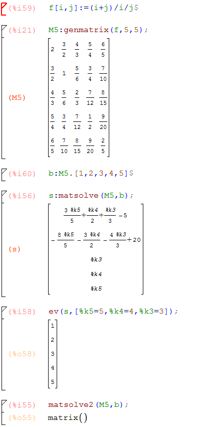
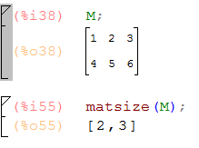
In Maxima, length(M) gives the number of rows, and so length(transpose(M)) gives the number of columns.  I put those together in a little widget matsize() that returns the list [m,n] for an m \times n matrix M:

matsize

matsize(A):=[length(A),length(transpose(A))];

Solving the matrix vector equation Ax=b in Maxima

*Upadate:  I’ve implemented a Maxima matrix-vector equation solver with simpler Maxima-specific algorithm in a later post.  That method is based on the built-in function linsolve().  In that post I show an example that breaks linsolve() but that is handled correctly by the backsolve() method.

Is there really not a solver in Maxima that takes matrix A and vector b and returns the solution of Ax=b ?  Of course we could do invert(A).b, but that ignores consistent systems where A isn’t invertible…or even isn’t square.

Here’s a little function matsolve(A,b)  that solves Ax=b for general A using the built-in Gaussian Elimination routine echelon(), with the addition of a homemade backsolve() function.  The function in turn relies on a little pivot column detector pivot() and my matrix dimension utility matsize(). This should include the possibilities of non-square A, non-invertible A, and treats the case of non-unique solutions in a more or less systematic way.

matsolve

matsolve(A,b):=block(
   [AugU],
   AugU:echelon(addcol(A,b)),
   backsolve(AugU)
 );

backsolve(augU):=block(
 [i,j,m,n,b,x,klist,k,np,nosoln:false],
 [m,n]:matsize(augU),
 b:col(augU,n),
 klist:makelist(concat('%k,i),i,1,n-1),
 k:0,
 x:transpose(matrix(klist)),
 for i:m thru 1 step -1 do (
   np:pivot(row(augU,i)), 
   if is(equal(np,n)) then
     (nosoln:true,return())
   else if not(is(equal(np,0))) then
     (x[np]:b[i],
     for j:np+1 thru n-1 do
       x[np]:x[np]-augU[i,j]*x[j])
    ),
 if nosoln then 
    return([])
 else 
   return(expand(x)) 
)$

matsize(A):=[length(A),length(transpose(A))]$

pivot(rr):=block([i,rlen],
 p:0,
 rlen:length(transpose(rr)),
 for i:1 thru rlen do( 
 if is(equal(part(rr,1,i),1)) then (p:i,return())), 
 return(p)
)$

Extracting Matrices from the Output of eigenvectors()

In class I sometimes need to use matrices of eigenvalues and eigenvectors, but the output of eigenvectors() isn’t particularly helpful for that out of the box.

Here are two one-liners that work in the case of simple eigenvalues.  I’ll post updates as needed:

First eigU(), takes the output of eigenvectors() and returns matrix of eigenvectors:

eigU(v):=transpose(apply('matrix,makelist(part(v,2,i,1),i,1,length(part(v,2)),1)));

And eigdiag(), which takes the output of eigenvectors() and returns diagonal matrix of eigenvalues:

eigdiag(v):=apply('diag_matrix,part(v,1,1));

eigs

For a matrix with a full set of eigenvectors but eigenvalues of multiplicity greater than one, the lines above fail.  A version of the above that works correctly in that case could look like:

eigdiag(v):=apply('diag_matrix,flatten(makelist(makelist(part(v,1,1,j),i,1,part(v,1,2,j)),j,1,length(part(v,1,1)))));

eigU(v):=transpose(apply('matrix,makelist(makelist(flatten(part(v,2))[i],i,lsum(i,i,part(v,1,2))*j+1,lsum(i,i,part(v,1,2))*j+lsum(i,i,part(v,1,2))),j,0,lsum(i,i,part(v,1,2))-1)));