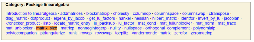
**Update** I didn’t find it it in documentation for quite a while, but there is a built-in Maxima function matrix_size() in the package linearalgebra that does what this little one-liner does**
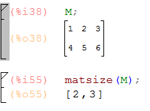
I really wanted a Maxima function that works something like MATLAB size() to easily determine the number of rows and columns for a matrix In Maxima, length(M) gives the number of rows, and so length(transpose(M)) gives the number of columns. I put those together in a little widget matsize() that returns the list [m,n] for an matrix
Is there really not a solver in Maxima that takes matrix A and vector b and returns the solution of ? Of course we could do invert(A).b, but that ignores consistent systems where isn’t invertible…or even isn’t square.
Here’s a little function matsolve(A,b) that solves for general using the built-in Gaussian Elimination routine echelon(), with the addition of a homemade backsolve() function. The function in turn relies on a little pivot column detector pivot() and my matrix dimension utility matsize(). This should include the possibilities of non-square , non-invertible , and treats the case of non-unique solutions in a more or less systematic way.
matsolve(A,b):=block(
   [AugU],
   AugU:echelon(addcol(A,b)),
   backsolve(AugU)
 );

backsolve(augU):=block(
 [i,j,m,n,b,x,klist,k,np,nosoln:false],
 [m,n]:matsize(augU),
 b:col(augU,n),
 klist:makelist(concat('%k,i),i,1,n-1),
 k:0,
 x:transpose(matrix(klist)),
 for i:m thru 1 step -1 do (
   np:pivot(row(augU,i)),
   if is(equal(np,n)) then
     (nosoln:true,return())
   else if not(is(equal(np,0))) then
     (x[np]:b[i],
     for j:np+1 thru n-1 do
       x[np]:x[np]-augU[i,j]*x[j])
    ),
 if nosoln then
    return([])
 else
   return(expand(x))
)$

matsize(A):=[length(A),length(transpose(A))]$

pivot(rr):=block([i,rlen],
 p:0,
 rlen:length(transpose(rr)),
 for i:1 thru rlen do(
 if is(equal(part(rr,1,i),1)) then (p:i,return())),
 return(p)
)$
In class I sometimes need to use matrices of eigenvalues and eigenvectors, but the output of eigenvectors() isn’t particularly helpful for that out of the box.
Here are two one-liners that work in the case of simple eigenvalues. I’ll post updates as needed:
First eigU(), takes the output of eigenvectors() and returns matrix of eigenvectors:
And eigdiag(), which takes the output of eigenvectors() and returns diagonal matrix of eigenvalues:
eigdiag(v):=apply('diag_matrix,part(v,1,1));
For a matrix with a full set of eigenvectors but eigenvalues of multiplicity greater than one, the lines above fail. A version of the above that works correctly in that case could look like:
Since 2011, Maxima has included the user-contributed numerical ODE solver rkf45() created by Panagiotis Papasotiriou. This implementation of the fourth (and fifth) order Runge-Kutta-Fehlberg embedded method features adaptive timestep selection and a nicely optimized function evaluation to make it run pretty fast in Maxima. As an explicit RK method, it is suitable for non-stiff equations. To use it in Maxima, you must first load(rkf45).
For years in my differential equations class, we’ve test-driven the various numerical ODE methods in MATLAB and explored their behavior on stiff systems. This year we’ve switched from MATLAB to Maxima, and I’ve written a stiff solver for that purpose. It’s an adaptive stepsize implementation of the second-order Backward Difference Formula. The BDF.mac file can be found here. The package contains a fixed-stepsize implementation BDF2() and the adaptive stepsize BDF2a().
I’ve tried to make the calling sequence and options as close to rkf45() as possible. I have not made any attempt to optimize the performance of the method. BDF methods are implicit, meaning that a nonlinear equation (or system of equations) must be solved at each step. For that I use the user-contributed Maxima function mnewton().
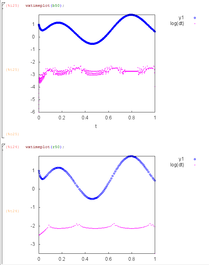
Additionally, note that I included my homemade help utility so that once BDF.mac is loaded, help(BDF2) and help(BDF2a) display help lines in the console window. For simplicity in comparing the methods, the load(rkf45) command is included in BDF.mac, as is an rkf45 help file for use with help(). Finally, I included in the package my little solution plotting utility wxtimeplot() which takes the “list of lists” output of BDF2(), BDF2a() and rkf45() and plots the dependent variables vs the independent variable along with a log-scale plot of the stepsize.
Below is an example that illustrates how the the BDF method performs relative to rkf45 for an increasingly stiff problem.
The equation is
For small values of , the explicit rkf method’s adaptive stepsizes result in much more efficient solutions for a given accuracy level. However for large the implicit BDF method is comparatively much more efficient, in terms of number of steps, and number of function evaluations, although in its current implementation, the BDF method takes more time.
Here’s the results for :
But for , the performance situation is reversed, with the BDF formula essentially immune from the effects of extra stiffness, while the rkf method requires an order of magnitude more steps.
I looked in the NASA archives for the work of Katherine Johnson described so dramatically in the film “Hidden Figures”. I found this 1960 paper:
In particular, I was struck by the film’s use of “Euler’s Method” as the critical plot point, and sadly couldn’t find anything about the use of that method in the archive, nor mention of it in the text of Margot Lee Shetterly’s book on which the film “Hidden Figures” is based.
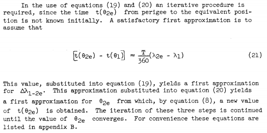
I did however read in the paper about an “iterative procedure” needed to solve for one variable.
Turns out the sequence of equations described in the report, when assembled into an expression in the single variable of interest, defines a contraction mapping and so converges by functional iteration, as is numerically demonstrated in the paper.
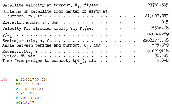
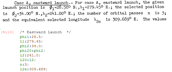
At the bottom I’ve linked a fuller treatment in a .wxmx file. Briefly, the authors describe the problem:
Here’s everything from the paper needed to do that in Maxima:
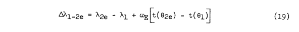
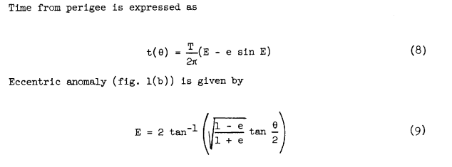
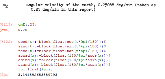
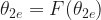
I put together equations 19,20,8, and 9, together with all those constants defined by the paper and customized trig function that act on angles measured in degrees, into an expression of the form
and applied the built-in Maxima numerical solver find_root(). The result agrees reasonably well with the result quoted in the paper.
In the above, I computed the derivative of the mapping evaluated at the solution and found that the value is much less than one, showing it is a contraction.
With over 300,000 downloads per year, Maxima is gaining popularity as a Computer Algebra System comparable to commercial systems like Mathematica and Maple.
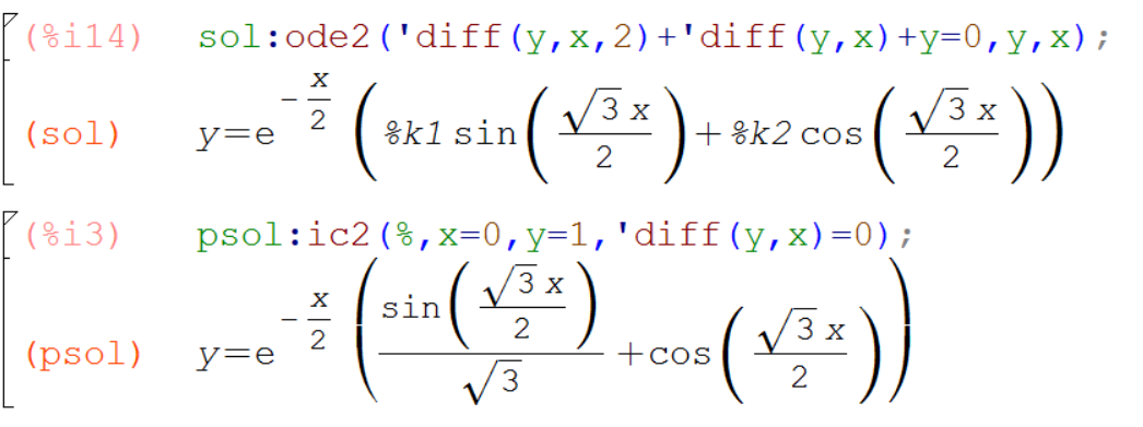
I was working on a differential equations homework problem and it took me a few tries to remember how to simplify a trig expression. So, I thought I’d put the results here to remind myself and others about trigexpand().
The second order linear equation is
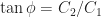
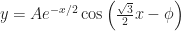
Now I asked my students to use the identities
and
to write the equation equivalently as
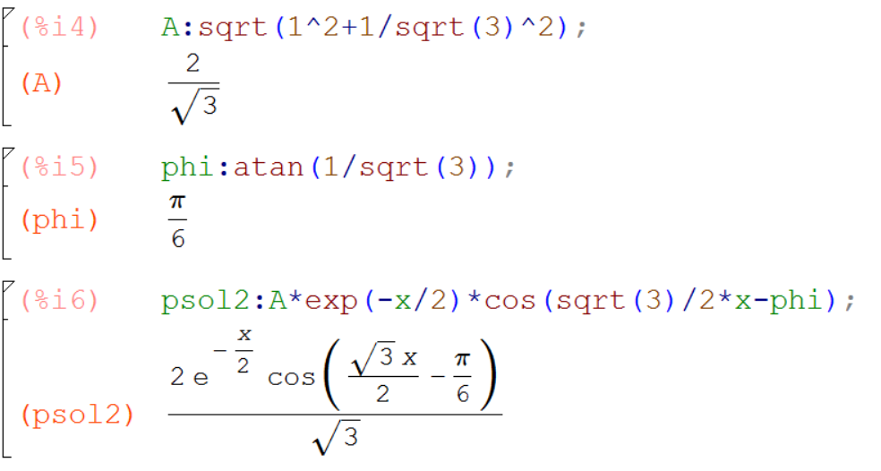
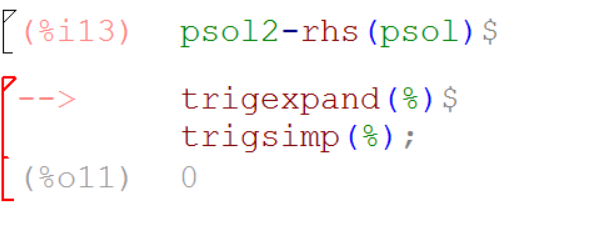
Finally, I wanted to use Maxima to show these two expressions are equivalent. I reflexively used trigsimp() on the difference between the two expression (the name says it all, am I right?) but the result was complicated in a way that I couldn’t recover…certainly not zero as I hoped. A few minutes of thought and I remembered trigexpand() which, followed by a call to trigsimp(), gives the proof:


 ? Of course we could do invert(A).b, but that ignores consistent systems where
  isn’t invertible…or even isn’t square.


 , the explicit rkf method’s adaptive stepsizes result in much more efficient solutions for a given accuracy level. However for large
  the implicit BDF method is comparatively much more efficient, in terms of number of steps, and number of function evaluations, although in its current implementation, the BDF method takes more time.
 :
:
 , the performance situation is reversed, with the BDF formula essentially immune from the effects of extra stiffness, while the rkf method requires an order of magnitude more steps.
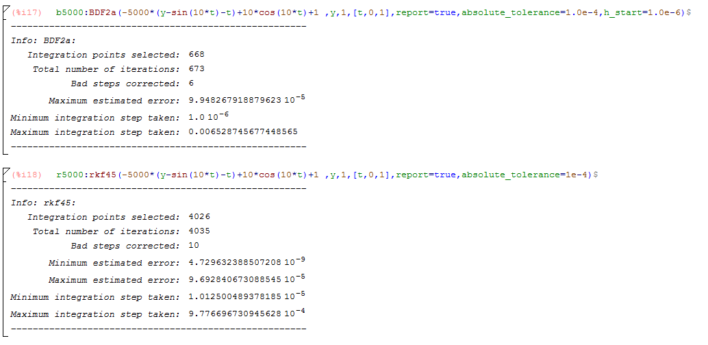


 quoted in the paper.
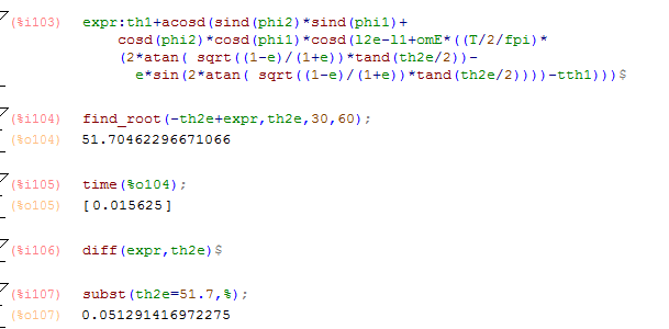
 evaluated at the solution and found that the value is much less than one, showing it is a contraction.
 and
and