trigexpand(), trigsimp() and an oscillatory solution of a 2nd order linear differential equation

I was working on a differential equations homework problem and it took me a few tries to remember how to simplify a trig expression.  So, I thought I’d put the results here to remind myself and others about trigexpand().

The second order linear equation is

 y''+y'+y=0 \;\;\;\;\;\; y(0)=1, y'(0)=0

odesol

Now I asked my students to use the identities

  A= \sqrt{C_1^2 + C_2^2}  and  \tan \phi=C_2/C_1

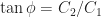
to write the equation equivalently as

 y=A e^{-x/2} \cos \left( \frac{\sqrt{3}}{2}  x -\phi \right)

odeoscillparams

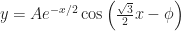
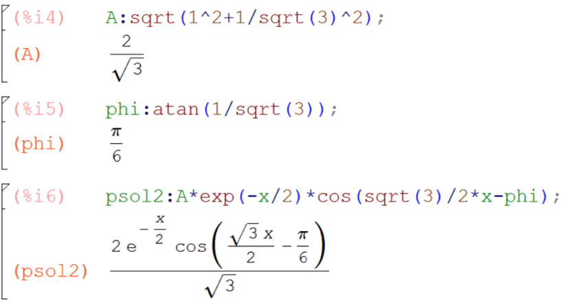
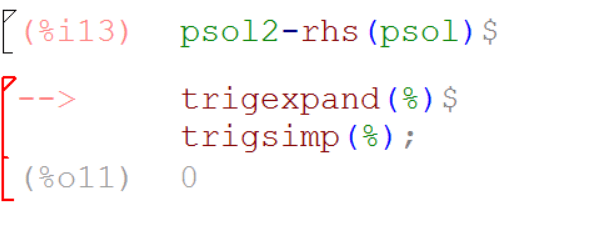
Finally, I wanted to use Maxima to show these two expressions are equivalent.  I reflexively used trigsimp() on the difference between the two expression   (the name says it all, am I right?)  but the result was complicated in a way that I couldn’t recover…certainly not zero as I hoped.  A few minutes of thought and I remembered trigexpand() which, followed by a call to trigsimp(), gives the proof:

odetrigexpand

Advertisement

Visualizing Complex Functions by their images over concentric circles

A few weeks ago I posted my Maxima code for visualizing complex function by their images over a grid of line segments in the complex plane.  Here are a few images from an experiment of plotting the image of complex function over concentric circles, centered at the origin, traversed in the counterclockwise direction.  The first image below shows the identity map.  The colors are in ROYGBIV rainbow order, as noted in the legend, which gives the radius of the pre-image circles.  The second image is for the function f(z)=(z-1/2)(z-1).  Notice for the smallest radius pre-image, the image under f is largely unchanged.  As radius grows the image forms a loop then doubles on itself.  Here’s a fun insight:  that looping behavior occurs at radius .75, a circle containing a point z at which f'(z)=0.  More on this later, but its exciting to find a geometric significance of a zero of the derivative, considering how much importance such points have in real calculus.  Finally the third figure shows really interesting behavior for the function f(z)=\frac{1}{(z-1/2)(z-1)}.  Notice again the looping brought about by points at which the derivative is zero.  Notice also the change in direction of the image each time we cross over a pole—that is a root of the denominator.  The maxima code is given below.
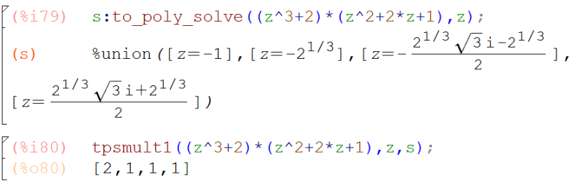
/* wxdrawcircleC
 plot the traces of complex valued function _f
 along concentric circles |z|=r for 0<r <=1
 blue - images of _f along horizontal lines
 red - images of _f along vertical lines */
wxdrawcircleC(_f):=block(
[fx,fy,fxt,fyt,pl,j,ncirc,r,theta_shift,lm,l,dx,dy,dxy,v,nt],
ratprint:false,
fx:realpart(rectform(subst(z=x+%i*y,_f))),
fy:imagpart(rectform(subst(z=x+%i*y,_f))),
pl:[],
nt:200,
r:2,
ncirc:7,
theta_shift:%pi/20,
/* get the max modulus for computing length of arrows */
lm:0,
for n:1 thru ncirc do (
l:cons(lm,makelist(cabs(subst(z=r*n/7*exp(%i*t),_f)),t,0,2*%pi,.5)),
 lm:lmax(l)
 ),
 for j:1 thru ncirc do(
 /*first the images of the circles */
 fxt:subst([x=r*cos(t)*j/ncirc,y=r*sin(t)*j/ncirc],fx),
 fyt:subst([x=r*cos(t)*j/ncirc,y=r*sin(t)*j/ncirc],fy),
 pl:cons([parametric(fxt,fyt,t,0,2*%pi)] , pl),
 pl:cons([color=colorlist(j)],pl),
 pl:cons([key=string(r*j/ncirc)],pl),
 /* now the arrows */
 dx:subst(t=3/nt,fxt)-subst(t=0,fxt),
 dy:subst(t=3/nt,fyt)-subst(t=0,fyt),
 dxy:sqrt(dx^2+dy^2),
 v:vector([subst(t=0,fxt),subst(t=0,fyt)],[lm*dx/dxy/20,lm*dy/dxy/20]),
 pl:cons([v],pl),
 pl:cons([head_length=lm,head_angle=1],pl),
 pl:cons([color=colorlist(j)],pl),
 pl:cons([key=""],pl)
 ),
pl:cons([xlabel="",ylabel=""],pl),
pl:cons([nticks=nt],pl),
pl:cons([grid=on],pl),
apply(wxdraw2d,pl)
);

Complex Factors of Real and Complex Polynomials – part 2

Last week I posted a Maxima utility to factor polynomials using complex roots.  The idea was to use the built-in solver solve to find each root a with multiplicity m, and then construct a factor of the form (z-a)^m.  Typically, solve can fail to identify some roots that are returned by the more robust to_poly_solve.  My problem at that time was that I didn’t know how to access the multiplicities for the roots returned by to_poly_solve.

I’ve written a utility to determine multiplicities for the roots returned by to_poly_solve. With that, here’s an updated version of factorC that takes advantage of the more robust solver.

/* factor a polynomial using all its complex roots */
factorC(_f,_z):=block(
[s,n,m,fp,j],
fp:1,
ss:to_poly_solve(_f,_z),
s:create_list(args(ss)[k][1],k,1,length(ss)),
m:tpsmult1(_f,_z,ss),
/*These lines were needed before I figured out how
 how to handle multiplicities with to_poly_solve
s:solve(_f,_z),
m:multiplicities,*/
n:length(s),
for j:1 thru n do 
 if lhs(s[j])#0 
 then fp:fp*(_z-(rhs(s[j])))^m[j],
 fp:fp*divide(_f,fp)[1],
fp
);

Roots, Multiplicities, and to_poly_solve

A few days ago I posted some code to factor and perform partial fraction decomposition using all available complex roots.  The approach is to find roots a — taking note of the multiplicity m of each —  and then construct factors of the form (z-a)^m.

As I’ve noted before, the built-in command solve can fail to find solutions.  The more robust Maxima solver is to_poly_solve.    That said, after a call to to_poly_solve, I don’t know how to get my hands on the multiplicities.  So, I’ve written a little utility to compute and return a list of multiplicities for the roots returned by to_poly_solve.  Here’s an example, followed by the code.  Notice that because to_poly_solve returns solutions using the %union construction, extracting the jth root requires something like root:rhs(part(s,j,1))

tpsmult1

/* tpsmult1 assumes results of to_poly_solve applied to _f, 
 are passed in the argument s */
tpsmult1(_f,_z,s):=block(
[d,root,nroots,mult,m1],
nroots:length(s),
mult:[],
for j:1 thru nroots do (
root:rhs(part(s,j,1)),
m1:rootmult(_f,_z,root),
mult: endcons(m1,mult)
),
mult
);

/* find the multiplicity of a root _a for the polynomial _f */
rootmult(_f,_z,_a):=block(
[d,val,m,mm],
m:1,
d:divide(_f,(_z-_a)),
val:subst(_z=_a,part(d,1)),
if (val=0) then (
 mm:rootmult(part(d,1),_z,_a),
 m:m+mm
 ),
m
);

Partial Fraction Decomposition Using Complex Factors

A few days ago I wrote about my solution for factoring a polynomial into factors corresponding to complex roots,  factorC.

One of the uses for that utility is to perform a partial fractions decomposition of rational functions.  Here’s a complex partial fraction function that uses factorC and the built-in Maxima function partfrac.

partfracC

partfracC(_f,_z):=block(
[d,fd],
d:denom(_f),
fd:factorC(d,_z),
partfrac(1/fd,_z)
);

Complex Factors of Real and Complex Polynomials

I’m getting ready for my fall Complex Variables class.  I noticed that the built-in Maxima function residue doesn’t reliably do the right thing.  My goal is to make some improvements to  Maxima residue calculations in Maxima over the course of the next month.

As I started to look at some test cases, I realized I didn’t know how to factor a polynomial into complex factors.  In the simplest case:

realfactor

but I wanted to see

manual_complexfactor

Maybe someone will find this and let me know that there’s a simple way to make that happen using existing Maxima commands.  Until then, I’ve written a little utility  to identify the roots (both real and complex) of a polynomial and return a factorization.  Here’s an example, and the code.  Notice that it only works as well as the root finder solve.  I tried to upgrade to the more robust to_poly_solve,  but I don’t yet know how to handle multiplicities in that case.

factorCexample

factorC(_f,_z):=block(
[s,n,m,fp,j],
fp:1,
/* This commented code was meant to use the
more robust solver to_poly_solve, but 
I couldn't understand how to handle multiplicities
ss:args(to_poly_solve(_f,_z)),
s:create_list(ss[k][1],k,1,length(ss)),*/
s:solve(_f,_z),
m:multiplicities,
n:length(s),
for j:1 thru n do 
 if lhs(s[j])#0 
 then fp:fp*(_z-(rhs(s[j])))^m[j],
 fp:fp*divide(_f,fp)[1],
fp
);