For the thoroughly modern calculus student, an introduction to Complex Variables is all the more daunting because we don’t have the kind of geometric intuition-building machinery available to us for functions 


/* plot the traces of complex valued function _f
 along grid lines in the square
 -1 <= Real(z) <= 1, -1<=Ima(z)<=1
 blue - images of _f along horizontal lines
 red - images of _f along vertical lines */
drawgridC(_f):=block(
[fx,fy,fxt,fyt,pl,j,ngrid],
fx:realpart(rectform(subst(z=x+%i*y,_f))),
fy:imagpart(rectform(subst(z=x+%i*y,_f))),
pl:[],
ngrid:19,
 for j:0 thru ngrid do(
 fxt:subst([x=-1+j*2/ngrid,y=t],fx),
 fyt:subst([x=-1+j*2/ngrid,y=t],fy),
 pl:cons([parametric(fxt,fyt,t,-1,1)] , pl)
 ),
pl:cons([color=red],pl),
 for j:0 thru ngrid do(
 fxt:subst([y=-1+j*2/ngrid,x=t],fx),
 fyt:subst([y=-1+j*2/ngrid,x=t],fy),
 pl:cons([parametric(fxt,fyt,t,-1,1)] , pl)
 ),
pl:cons([color=blue],pl),
pl:cons([xlabel="",ylabel=""],pl),
pl:cons([nticks=200],pl),
apply(wxdraw2d,pl)
);
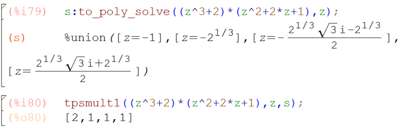
 with multiplicity
  , and then construct a factor of the form
  . Typically, solve can fail to identify some roots that are returned by the more robust to_poly_solve. My problem at that time was that I didn’t know how to access the multiplicities for the roots returned by to_poly_solve.
 th root requires something like root:rhs(part(s,j,1))