For my multivariable calculus class, I wanted an easy-to-call suite of symbolic integrators for path integrals of the form
 ,
,
 , or
, or
 .
.
My overarching design idea was that the input arguments needed to look the way they do when I teach the course:
- a scalar field
 or a vector field
  or
or 
- a curve
 defined by a vector-valued function
  where
where  as appropriate.
It took me a while to work out how to evaluate the integrand along the path within my function. Things that worked fine on the command line failed when embedded into a batch file to which I passed functions as arguments. I ended up using subst, one variable at a time. I’d like to be able to do this in a single command which can detect whether we’re in 2 or 3 dimensions so that I don’t need separate commands.
For now, here’s what I came up with along with some illustrative examples taken from Paul’s online math notes, that show how to call these new commands I, I2 and I3.
/* path integral of a scalar integrand f(x,y) on path r(t) in R^2, t from a to b */
 I(f,r,t,a,b):=block(
 [f1,f2,dr,Iout],
 f1:subst(x=r[1],f),
 f2:subst(y=r[2],f1),
 dr:sqrt(diff(r,t).diff(r,t)),
 Iout: integrate(f2*dr,t,a,b),
 Iout
 );
/* path integral of a vector integrand F(x,y) on path r(t) in R^2, t from a to b */
 I2(H,r,t,a,b):=block(
 [H1,H2,I],
 H1:subst(x=r[1],H),
 H2:subst(y=r[2],H1),
 I: integrate( H2.diff(r,t),t,a,b),
 I
 );
/* path integral of a vector integrand F(x,y,z) on path r(t) in R^3, t from a to b */
 I3(H,r,t,a,b):=block(
 [H1,H2,H3,I],
 H1:subst(x=r[1],H),
 H2:subst(y=r[2],H1),
 H3:subst(z=r[3],H2),
 I: integrate( H3.diff(r,t),t,a,b),
 I
 );

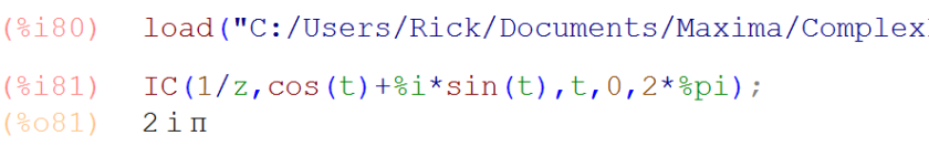
Here’s an update: a related maxima function for evaluating a complex integral

where  and the curve
  is given by
  .
.
/* path integral of a complex integrand f(z): C --> C, on path z(t): R --> C, t from a to b */
IC(f,r,t,a,b):=block(
[f1,dz,Iout],
f1:subst(z=r,f),
dz:diff(r,t),
Iout: integrate(f1*dz,t,a,b),
Iout
);


 . Notice for the smallest radius pre-image, the image under
  is largely unchanged. As radius grows the image forms a loop then doubles on itself. Here’s a fun insight: that looping behavior occurs at radius .75, a circle containing a point
  . More on this later, but its exciting to find a geometric significance of a zero of the derivative, considering how much importance such points have in real calculus. Finally the third figure shows really interesting behavior for the function
  . Notice again the looping brought about by points at which the derivative is zero. Notice also the change in direction of the image each time we cross over a pole—that is a root of the denominator. The maxima code is given below.


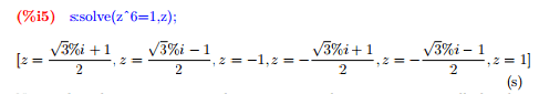
 with multiplicity
  , and then construct a factor of the form
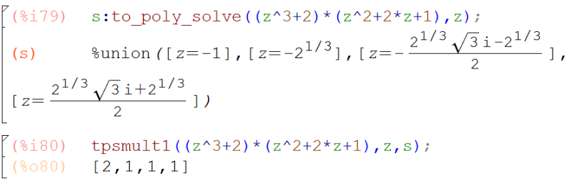
  . Typically, solve can fail to identify some roots that are returned by the more robust to_poly_solve. My problem at that time was that I didn’t know how to access the multiplicities for the roots returned by to_poly_solve.
 th root requires something like root:rhs(part(s,j,1))