
Look what I found in the share/contrib directory:

There isn’t any documentation available from texinfo:

Browsing around on the web I found this documentation page.
There are also many examples given in the Eulix_*.mac files in share/contrib/Eulix . Here’s what is says at the top of Eulix.mac:
* (C) Helmut Jarausch
 *
 * @version 1.0 Date August 29th, 2017
 *
 * @author Helmut Jarausch
 *         RWTH Aachen University

 * @contents
 *  Eulix is an linearly implicit (by default) extrapolated Euler method.
 *  It uses variable step sizes, variable orders and offers dense output.
 *  Eulix can solve systems like  M y'(t)= f(t,y)  where M is a constant mass
 *  matrix. This enables the solution of differential algebraic equations (DAE)
 *  of index 1, as well.
 *
 *  I have made a simplified version of  SEULEX  published in
 *
 *  E. Hairer, G.Wanner
 *  Solving Ordinary Differential Equations II
 *  Stiff and Differential-Algebraic Problems
 *  Springer 1991
A Test Problem: The Ball of Flame
To test drive the method, I’ll retrace Cleve Moler’s steps in this excellent piece about numerical solvers for stiff equations.
We’ll consider the “ball of flame” equation of Lawrence Shampine:
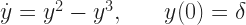
on the time interval 
The equation is meant to be a simple model of flame propagation, but it could also describe what happens to non-stiff solvers for small values of 
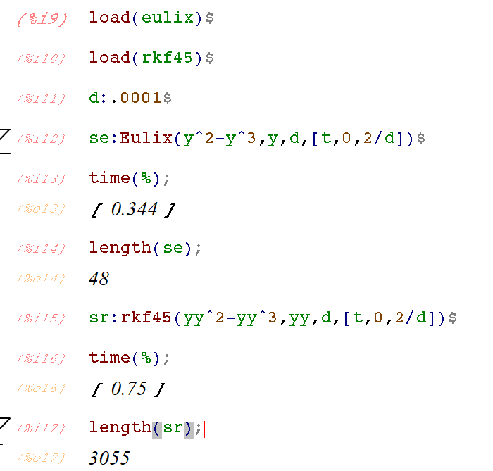
Notice that the basic calling sequence for Eulix() is the same as for rkf45(). The first thing to observe is that when applied to the ball of flame, Eulix() uses less time and less steps than rkf45():
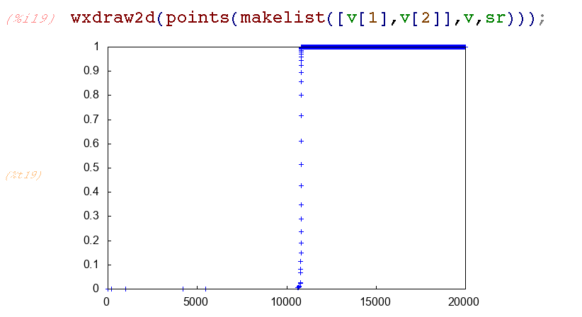
Plots of the solution points show that Eulix() makes this look like an easy problem, using very few points for the horizontal parts of the solution, and concentrating more points at the sharp turns:

The non-stiff variable step Runge-Kutta-Fehlberg method rkf45() makes this look hard:
Zooming in shows how hard rfk45() is working on the horizontal part of the solution. It is doing its job to maintain the error within the default tolerance 1e-6, but it’s using a lot of steps and function evaluations to do that:

And one final thing to know about Eulix(): The output can appear very sparse, as we see in the region 
Thank you Helmut Jarausch!
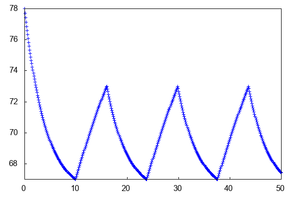

 when the cooling sytem is running, becomes zero if the system is running and the temperature reaches 67F, becomes 1 if the system is not running and the temperature reaches 73F. The behavior of the room temperature is shown in the figure at the top of this piece.
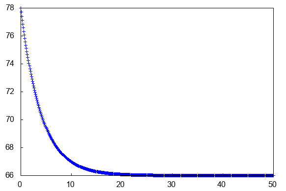


 ,
,  ,
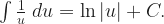
, ) in one step to use the antiderivative

 , but still…
 ,
, 


