Differential Equations – Page 2

A Package of Maxima Utilities for my Ordinary Differential Equations Course: MATH280.mac

I’ve put together a collection of functions — some direct quotes of other contributed functions, some renamed or repackaged, and some newly implemented — for various needed tasks in my undergraduate ordinary differential equations course.

I’ve written elsewhere about the Backward Difference Formula implementations, the phase space visualization functions, the matrix extractors, and the numerical solutions plotters.

The package includes my home-grown help utility.

You can download the package MATH280.mac

…and if you’re interested, here’s my multivariable calculus package MATH214.mac

MATH280.mac contains:
 wxphaseplot2d(s)
 wxphaseplot3d(s)
 phaseplot3d(s)
 wxtimeplot(s)
 plotdf(rhs)
 wxdrawdf(rhs)
 sol_points(numsol,nth,mth)
 rkf45(oderhs,yvar,y0,t_interval)
 BDF2(oderhs,yvar,y0,t_interval)
 BDF2a(oderhs,yvar,y0,t_interval)
 odesolve(eqn,depvar,indvar)
 ic1(sol,xeqn,yeqn)
 ic2(sol,xeqn,yeqn,dyeqn)
 eigU(z)
 eigdiag(z)
 clear()
 -
 -
 for any of the above functions,
 help(function_name) returns help lines for function_name
 -
 Last Modified 5:00 PM 3/27/2017

Plotting Numerical Solutions of Ordinary Differential Equations in Maxima

Maxima comes with a few well-implemented numerical ODE solvers — rk() and rkf45() — and I’ve written in a previous post about my variable stepsize implementation of the 2nd order backward differentiaion formula for stiff systems BDF2a().

Plotting the resulting numerical solutions — which is a list of lists of the form

[[indvar, depvar1, depvar2,… ], [indvar, depvar1, depvar2,… ], … ]

with each of the sublists representing the state of the system at a discrete time — requires a little familiarity with list functions like makelist() and map().

Here are a few little helper routines to make that quicker:

wxtimeplot()
wxphaseplot2d, wxphaseplot3d
sol_points()

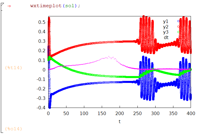
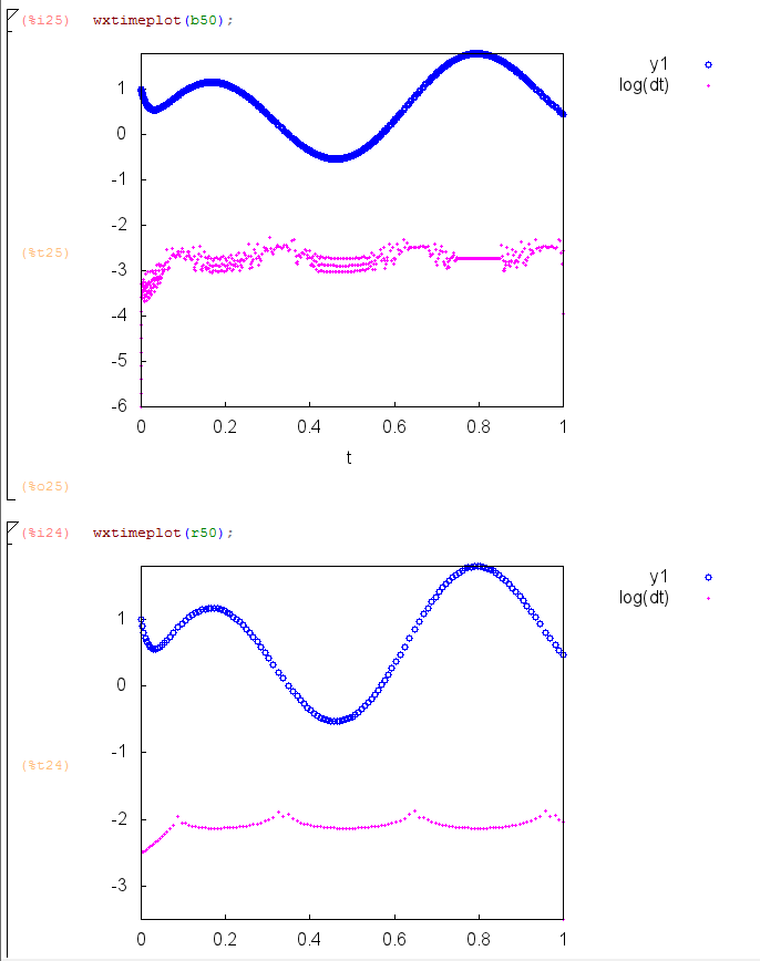
wxtimeplot()

This is mainly a teaching tool for my ordinary differential equations course, taking the output of the solver and, assuming there aren’t more than three dependent variables, plotting all the dependent variables vs the independent variable on the same set of axes, with a representation of the step size.

wxtimeplot

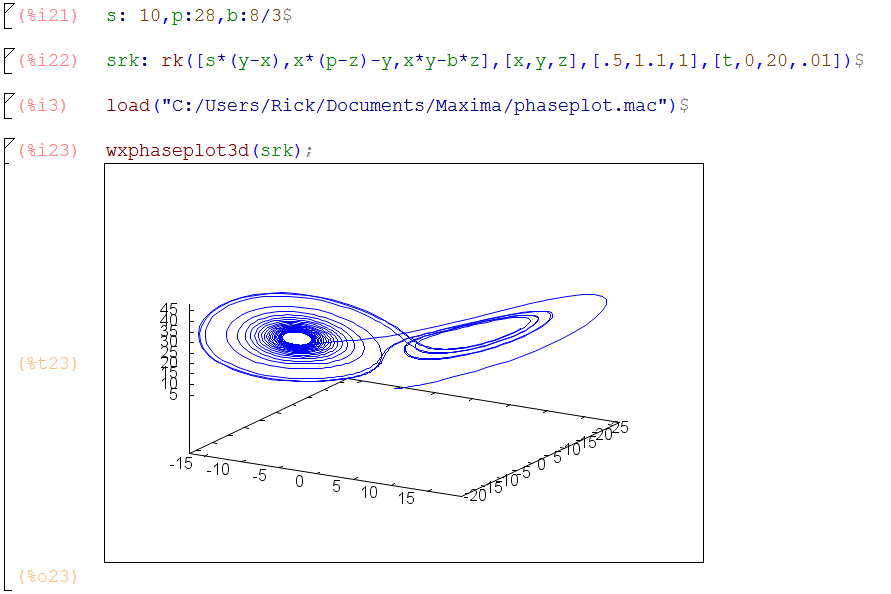
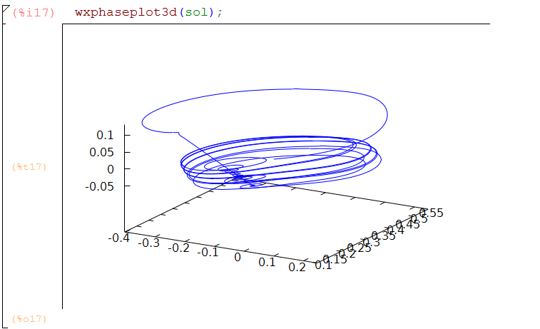
wxphaseplot2d,wxphaseplot3d

I wrote about these in another post

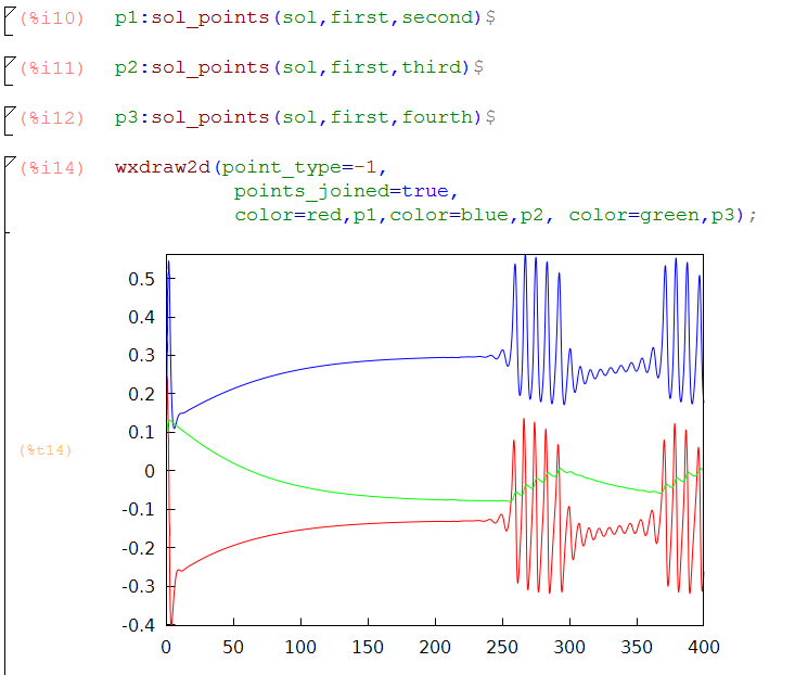
wxphaseplot3d

sol_points()

This is a more general purpose function. Given the output of the numerical ode solver, this constructs a points() subcommand ready to plug into draw2d(). This allows for the full generality of draw2d: colors, axis labels, point points,

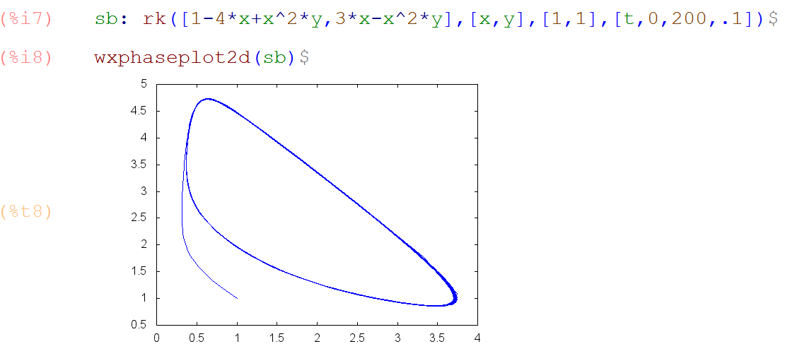
Especially useful for plotting results from more than one call to the solver, such as when we need to see the effect of changing a parameter value:

sol_points

Below I’ve pasted the code for the plots, and also for the interesting differential equations from Larter et al in Chaos, V.9 n.3 (1999)

(tw:(cosh((Vi-V3)/(2*V4))^(-1)),
m:(1/2)*(1+tanh((Vi-V1)/V2)),
w:(1/2)*(1+tanh((Vi-V3)/V4)),
aexe:aexe1*(1+tanh(Vi-V5)/V6),
ainh:ainh1*(1+tanh((Zi-V7)/V6))
)$

(rhs1:-gCa*m*(Vi-1)-gK*Wi*(Vi-ViK)-gL*(Vi-VL)+I-ainh*Zi,
 rhs2:(phi*(w-Wi)/tw),
 rhs3:b*(c*I+aexe*Vi)
 )$ 

(V1:-.01,V2:0.15,V3:0,V4:.3,V5:0,V6:.6,V7:0,
 gCa:1.1,gK:2,gL:0.5,VL:-.5,ViK:-.783,phi:.7,tw:1,
 b:0.0809,c:0.22,I:0.316,aexe1:0.6899,ainh1:0.695)$

 load(rkf45);

 sol:rkf45([''rhs1,''rhs2,''rhs3],[Vi,Wi,Zi],[.1,.1,.1],[t,0,400],
             report=true,absolute_tolerance=1e-8)$

sol_points(numsol,nth,mth):=points(map(nth,numsol),map(mth,numsol));

/* wxtimeplot takes the output of sol: rk45 and plots 
 up to 3 dependent variables 
plus the scaled integration step size vs time*/
wxtimeplot(sol):=block(
[t0,t,tt,dt,big,dtbig],
t0:map(first,sol),
t:part(t0,allbut(1)),
tt:part(t0,allbut(length(t0))),
dt:t-tt,
dtbig:lmax(dt),
big:lmax(map(second,abs(sol))),
if is(equal(length(part(sol,1)),3)) then(
 big: max(big,lmax(map(third,abs(sol)))),
 wxdraw2d(point_type=6, key="y1",
 points(makelist([p[1],p[2]],p,sol)),
 color=red, key="y2",
 points(makelist([p[1],p[3]],p,sol)),
 color=magenta, key="dt",point_size=.2,
 points(t,big*dt/dtbig/4),xlabel="t",ylabel=""))
elseif is(equal(length(part(sol,1)),2)) then
 wxdraw2d(point_type=6, key="y1",
 points(makelist([p[1],p[2]],p,sol)),
 color=magenta, key="dt",point_size=.2,
 points(t,big*dt/dtbig/4),xlabel="t",ylabel="")
elseif is(equal(length(part(sol,1)),4)) then(
 big: max(big,lmax(map(third,abs(sol)))),
 big: max(big,lmax(map(fourth,abs(sol)))),
 wxdraw2d(point_type=6, key="y1",
 points(makelist([p[1],p[2]],p,sol)),
 color=red, key="y2",
 points(makelist([p[1],p[3]],p,sol)),
 color=green, key="y3",
 points(makelist([p[1],p[4]],p,sol)),
 color=magenta, key="dt",point_size=.2,
 points(t,big*dt/dtbig/4),xlabel="t",ylabel=""))
 );

Extracting Matrices from the Output of eigenvectors()

In class I sometimes need to use matrices of eigenvalues and eigenvectors, but the output of eigenvectors() isn’t particularly helpful for that out of the box.

Here are two one-liners that work in the case of simple eigenvalues. I’ll post updates as needed:

First eigU(), takes the output of eigenvectors() and returns matrix of eigenvectors:

eigU(v):=transpose(apply('matrix,makelist(part(v,2,i,1),i,1,length(part(v,2)),1)));

And eigdiag(), which takes the output of eigenvectors() and returns diagonal matrix of eigenvalues:

eigdiag(v):=apply('diag_matrix,part(v,1,1));

eigs

For a matrix with a full set of eigenvectors but eigenvalues of multiplicity greater than one, the lines above fail. A version of the above that works correctly in that case could look like:

eigdiag(v):=apply('diag_matrix,flatten(makelist(makelist(part(v,1,1,j),i,1,part(v,1,2,j)),j,1,length(part(v,1,1)))));

eigU(v):=transpose(apply('matrix,makelist(makelist(flatten(part(v,2))[i],i,lsum(i,i,part(v,1,2))*j+1,lsum(i,i,part(v,1,2))*j+lsum(i,i,part(v,1,2))),j,0,lsum(i,i,part(v,1,2))-1)));

BDF2a: An adaptive-stepsize Stiff ODE solver in Maxima

**March 2021 update** Maxima has a full-featured stiff solver called Eulix now, thanks to Helmut Jarausch.

***************************************************

Since 2011, Maxima has included the user-contributed numerical ODE solver rkf45() created by Panagiotis Papasotiriou. This implementation of the fourth (and fifth) order Runge-Kutta-Fehlberg embedded method features adaptive timestep selection and a nicely optimized function evaluation to make it run pretty fast in Maxima. As an explicit RK method, it is suitable for non-stiff equations. To use it in Maxima, you must first load(rkf45).

For years in my differential equations class, we’ve test-driven the various numerical ODE methods in MATLAB and explored their behavior on stiff systems. This year we’ve switched from MATLAB to Maxima, and I’ve written a stiff solver for that purpose. It’s an adaptive stepsize implementation of the second-order Backward Difference Formula. The BDF.mac file can be found here. The package contains a fixed-stepsize implementation BDF2() and the adaptive stepsize BDF2a().

I’ve tried to make the calling sequence and options as close to rkf45() as possible. I have not made any attempt to optimize the performance of the method. BDF methods are implicit, meaning that a nonlinear equation (or system of equations) must be solved at each step. For that I use the user-contributed Maxima function mnewton().

Additionally, note that I included my homemade help utility so that once BDF.mac is loaded, help(BDF2) and help(BDF2a) display help lines in the console window. For simplicity in comparing the methods, the load(rkf45) command is included in BDF.mac, as is an rkf45 help file for use with help(). Finally, I included in the package my little solution plotting utility wxtimeplot() which takes the “list of lists” output of BDF2(), BDF2a() and rkf45() and plots the dependent variables vs the independent variable along with a log-scale plot of the stepsize.

Below is an example that illustrates how the the BDF method performs relative to rkf45 for an increasingly stiff problem.

The equation is

$\dot{y} = -\lambda (y-\sin (10t)-t)+10 \cos (10t)+1 .$

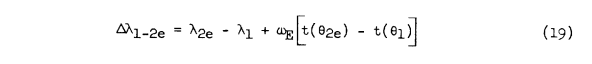
For small values of $\lambda$ , the explicit rkf method’s adaptive stepsizes result in much more efficient solutions for a given accuracy level. However for large $\lambda$ the implicit BDF method is comparatively much more efficient, in terms of number of steps, and number of function evaluations, although in its current implementation, the BDF method takes more time.

Here’s the results for $\lambda=50$ :

But for $\lambda=5000$ , the performance situation is reversed, with the BDF formula essentially immune from the effects of extra stiffness, while the rkf method requires an order of magnitude more steps.

References:

E. Alberdi Celaya , J. J. Anza Aguirrezabala , and P. Chatzipantelidis. “Implementation of an adaptive BDF2 formula and comparison with the MATLAB Ode15s”, Procedia Computer Science, December 2014

Using Maxima To Do Some Math Described in the Movie “Hidden Figures”

I looked in the NASA archives for the work of Katherine Johnson described so dramatically in the film “Hidden Figures”. I found this 1960 paper:

In particular, I was struck by the film’s use of “Euler’s Method” as the critical plot point, and sadly couldn’t find anything about the use of that method in the archive, nor mention of it in the text of Margot Lee Shetterly’s book on which the film “Hidden Figures” is based.

I did however read in the paper about an “iterative procedure” needed to solve for one variable.

Turns out the sequence of equations described in the report, when assembled into an expression in the single variable of interest, defines a contraction mapping and so converges by functional iteration, as is numerically demonstrated in the paper.

At the bottom I’ve linked a fuller treatment in a .wxmx file. Briefly, the authors describe the problem:

Here’s everything from the paper needed to do that in Maxima:

I put together equations 19,20,8, and 9, together with all those constants defined by the paper and customized trig function that act on angles measured in degrees, into an expression of the form

$\theta_{2e}=F(\theta_{2e})$

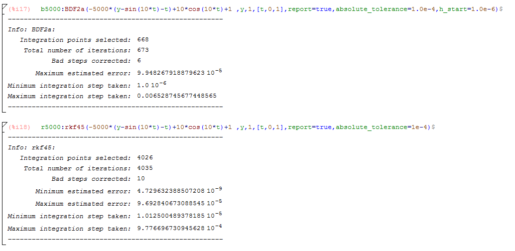
and applied the built-in Maxima numerical solver find_root(). The result agrees reasonably well with the result $\theta_{2e}=50.806$ quoted in the paper.

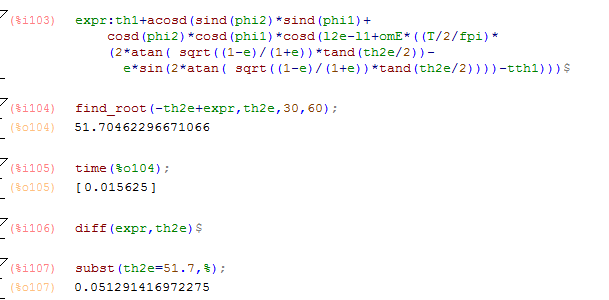
In the above, I computed the derivative of the mapping $F$ evaluated at the solution and found that the value is much less than one, showing it is a contraction.

Here’s my full wxMaxima session.

trigexpand(), trigsimp() and an oscillatory solution of a 2nd order linear differential equation

I was working on a differential equations homework problem and it took me a few tries to remember how to simplify a trig expression. So, I thought I’d put the results here to remind myself and others about trigexpand().

The second order linear equation is

$y''+y'+y=0 \;\;\;\;\;\; y(0)=1, y'(0)=0$

odesol

Now I asked my students to use the identities

$A= \sqrt{C_1^2 + C_2^2}$ and $\tan \phi=C_2/C_1$

to write the equation equivalently as

$y=A e^{-x/2} \cos \left( \frac{\sqrt{3}}{2} x -\phi \right)$

odeoscillparams

Finally, I wanted to use Maxima to show these two expressions are equivalent. I reflexively used trigsimp() on the difference between the two expression (the name says it all, am I right?) but the result was complicated in a way that I couldn’t recover…certainly not zero as I hoped. A few minutes of thought and I remembered trigexpand() which, followed by a call to trigsimp(), gives the proof:

odetrigexpand

Speeding Up Maxima Functions with compile()

In my differential equations class, we implement the first-order-accurate Euler method for numerical approximation of a solution of the initial value problem $y' = f(x,y)$ , $y(x_0)=y_0$ .

We implement this in an appealing way — from an algorithm translation point of view — but the inner loop with all that list indexing takes a lot of time. To verify the accuracy of the method, we run the function with more and more successively smaller steps.

eulermethod(f,x0,y0,h,nsteps):=block(
 [i,x,y], 
 x:makelist(0,i,1,nsteps+1,1),
 y:makelist(0,i,1,nsteps+1,1),
 x[1]:x0,
 y[1]:y0,
 for i:1 thru nsteps do (
    x[i+1]:x[i]+h,
    y[i+1]:y[i]+h*ev(f,x=x[i],y=y[i])
 ),
 return ([x,y])
)$

Below I’ve used the time() function so you can see how simply running compile() on the function makes it run lots faster for ten thousand steps!

The Maxima documentation says this:

Function: compile
compile (f_1, …, f_n)
compile (functions)
compile (all)

Translates Maxima functions f_1, …, f_n into Lisp, evaluates the Lisp translations, and calls the Lisp function COMPILE on each translated function. compile returns a list of the names of the compiled functions.

compile (all) or compile (functions) compiles all user-defined functions.

compile quotes its arguments; the quote-quote operator '' defeats quotation.

Compiling a function to native code can mean a big increase in speed and might cause the memory footprint to reduce drastically. Code tends to be especially effective when the flexibility it needs to provide is limited. If compilation doesn’t provide the speed that is needed a few ways to limit the code’s functionality are the following:

If the function accesses global variables the complexity of the function can be drastically be reduced by limiting these variables to one data type, for example using mode_declare or a statement like the following one: put(x_1, bigfloat, numerical_type)

The compiler might warn about undeclared variables if text could either be a named option to a command or (if they are assigned a value to) the name of a variable. Prepending the option with a single quote ' tells the compiler that the text is meant as an option.

Here are the specs of the machine I ran these timings on:

Maxima Language Code Translations

Have you seen these sites?

Hyperpolyglot.org and Rosettacode.org provide a valuable help for users who need to solve a problem in a new language: Line-by-line comparisons with lots of other languages.

For Maxima users, Hyperpolyglot’s computer-algebra system section has side-by-side tables of comparisons with Mathematica, Maple, Sage and Numpy.

Rosettacode is arranged by task, with user-contributed solutions to common tasks in lots of languages. I was motivated to write this post while working on a new Maxima version of an ordinary differential equations course I’ve taught for years using MATLAB.

Here is Rosettacode’s section on the Euler Method — a method for numerical approximation to the solution of a first order ordinary differential equation.

For the record, this is the version I decided to teach in my course:

(    /* Euler Method for  initial value problem
          y'=xy ,  y(0)=0.5   */ 
x0:0,
y0:.5,
h:.25,
nsteps:10,
xeuler:makelist(0,i,1,nsteps+1,1),
yeuler:makelist(0,i,1,nsteps+1,1),          
xeuler[1]:x0,
yeuler[1]:y0,
for i:1 thru nsteps do (
     xeuler[i+1]:xeuler[i]+h,
     yeuler[i+1]:yeuler[i]+h*xeuler[i]*yeuler[i]  
     )                                        
);

Checking the order of accuracy for the built-in ODE solver rk

The Maxima documentation says the numerical ODE solver in the command rk() is fourth order accurate. I ran a little test to confirm that.

Here’s the html export of the Maxima session, and a screenshot of the punchline:

RKorder4

Numerical Solutions of 2D and 3D ODE systems and phase plots

I most often use the built-in solvers in MATLAB (or the freeware alternative FreeMat) for numerical solutions of ODE systems. They are easy to call and MATLAB graphical output is very flexible and of high quality. That said, if I’m already working in Maxima to study stability behavior and equilibrium solutions, it’s fun to stay in the same window for a numerical solution.

Here’s an example: a damped, driven hard spring oscillator, written in phase space variables

$\dot{y}=z, \dot{z}=-y^3-y-z/10 + 3/10\cos(t)$

It’s straight-forward enough to run the Maxima numerical solver rk on this equation. Extracting the numerical values of the two dependent variables is a little bit of a drag, requiring a call to makelist. To make a plot in phase space, here’s a one-line function that is so easy to call:

/* wxphaseplot2d takes the output of s: rk([rhs1,rhs2]) 
   and  plots in phase space */
wxphaseplot2d(s):=wxplot2d([discrete,makelist([p[2],p[3]],p,s)],[xlabel,""],[ylabel,""]);

Here’s how it works on the above example with a cute phase-space solution curve:

phaseheart

And here’s another famous phase curve—the solution of the Brusselator:

brusselatorphase

And can I just point out how analytically solving for the equilibrium solution has a very similar calling sequence — so easy that there’s no reason not to do it every time you want a numerical solution, and vice versa!

brusselator_eqsoln

Update! Here’s a 3D phase plotter

/* wxphasplot3d takes the output of s: rk([rhs1,rhs2,rhs3]) and plots in phase space */

wxphaseplot3d(s):=wxdraw3d(point_type=0,point_size=.3,points_joined=true,points(makelist([p[2],p[3],p[4]],p,s)));

A classical example of 3D phase space trajectory curves, the Lorenz strange attractor system:

lorenz3D

	Rick on An improved Maxima function fo…
	adrian on An improved Maxima function fo…
	Extracting matrices… on Extracting Matrices from the O…
	Matthew Pettis on Functions, :, and :=
	warrena623 on Legend Position in Maxima…