Tag: Stiffness

**March 2021 update** Maxima has a full-featured stiff solver called Eulix now, thanks to Helmut Jarausch.

***************************************************

Since 2011, Maxima has included the user-contributed numerical ODE solver rkf45() created by Panagiotis Papasotiriou.  This implementation of the fourth (and fifth) order Runge-Kutta-Fehlberg embedded method features adaptive timestep selection and a nicely optimized function evaluation to make it run pretty fast in Maxima.  As an explicit RK method, it is suitable for non-stiff equations.  To use it in Maxima, you must first load(rkf45).

For years in my differential equations class, we’ve test-driven the various numerical ODE methods in MATLAB and explored their behavior on stiff systems.  This year we’ve switched from MATLAB to Maxima, and I’ve written a stiff solver for that purpose.  It’s an adaptive stepsize  implementation of the second-order Backward Difference Formula.  The BDF.mac file can be found here.  The package contains a fixed-stepsize implementation BDF2()  and the adaptive stepsize BDF2a().

I’ve tried to make the calling sequence and options as close to rkf45() as possible.  I have not made any attempt to optimize the performance of the method.  BDF methods are implicit, meaning that a nonlinear equation (or system of equations) must be solved at each step.  For that I use the user-contributed Maxima function mnewton().

Additionally, note that I included my homemade help utility so that once BDF.mac is loaded, help(BDF2) and help(BDF2a) display help lines in the console window. For simplicity in comparing the methods, the load(rkf45) command is included in BDF.mac, as is an rkf45 help file for use with help().   Finally, I included in the package my little solution plotting utility wxtimeplot() which takes the “list of lists” output of BDF2(), BDF2a() and rkf45() and plots the dependent variables vs the independent variable along with a log-scale plot of the stepsize.

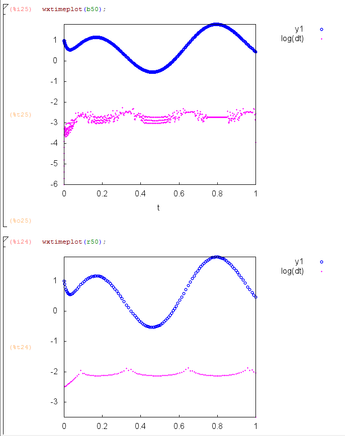
Below is an example that illustrates how the the BDF method performs relative to rkf45 for an increasingly stiff problem.

The equation is

For small values of , the explicit rkf method’s adaptive stepsizes result in much more efficient solutions for a given accuracy level.  However for large the implicit BDF method is comparatively much more efficient, in terms of number of steps, and  number of function evaluations, although in its current implementation, the BDF method takes more time.

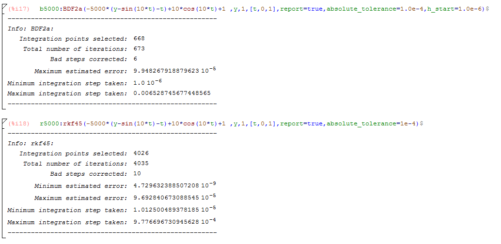
Here’s the results for :

But for , the performance situation is reversed, with the BDF formula essentially immune from the effects of extra stiffness, while the rkf method requires an order of magnitude more steps.

References:

E. Alberdi Celaya , J. J. Anza Aguirrezabala , and P. Chatzipantelidis.  “Implementation of an adaptive BDF2 formula and comparison with the MATLAB Ode15s”,  Procedia Computer Science,  December 2014