$latex \int x^2 dx$

I’m testing the latex math-mode utility in WordPress.com.  The first thing to know is that based on the way the title of this post appears, the latex utility doesn’t work in post titles.

The rub here is that MathJax would be the natural solution, but WordPress.com isn’t compatible with JavaScript.  

That leaves us with $, followed by the word latex, followed by my latex markup, followed by a closing $ , which I illustrate  below with a screenshot because I don’t know how to quote a string verbatim in WordPress:

preform

This works OK as inline style math \int x^2 dx and I think we could simulate display math mode like this with manual paragraph centering and with the optional size argument &s=1 inside the dollar signs (the default size is 0)

\int x^2 dx

and then back to inline for f(x).

And there it is.

The official guide to the  WordPress \LaTeX utility  can be found here.

Functions, :, and :=

I’m really posting this for myself to act as a big paperweight.  Whenever I forget about :=  and : for functions in Maxima, I can refer to this page.

The gist:

  • g(x):=x^2  results in a function you can evaluate as g(3)
  • f: x^2 results in an expression you can evaluate with ev(f,x=3)
  • ev works with both:  ev(g(x),x=3)  or ev(f,x=3)
  • also subst(x=3,f) and subst(x=3,g(x))
  • based on our definition, g doesn’t have a meaning…only  g(x) does
  • likewise, f(3) doesn’t have a meaning here…only the symbol f does
  • finally h:=x^2 gives an error — explicit dependent variable needed with :=

colonequals

subst

colonequalserror

A few notes about exporting to .tex in Windows

23 March, 2016 Update!  The following was true for my windows installation of version wxMaxima 15.8.1-git.  I’ve just updated to wxMaxima 15.8.2 64 bit windows version and all is as expected — put TeX: at the beginning of the each text cell, then write latex like a boss.  I’m still not using dollar signs, for compatibility with mathJax when I export to html format 🙂


I really became a believer in the usefuless of Maxima as a productive part of my (and my students) workflow because of the easy way wxMaxima allows the user to document their work in an html or pdf (via pdflatex) document that include LaTeX markup for beautiful mathematical notation.

On my linux machine (Ubuntu 14.04) exporting my wxMaxima session to .tex behaves pretty nicely — maybe I’ll make a future post about that.  In particular, simply putting the string “TeX:” at the beginning of the document allows free use of LaTeX markup to be correctly rendered in the exported .tex document.  This doesn’t work in my Windows version, as well as a few other things described here.

In this post, I’ll describe what I’ve been doing to work around the problems in .tex export in Windows while being consistent with typesetting markups that make for good-looking HTML exports as well.

Goodbye dollar signs

After 25 years of using $…$ for inline math mode and $$…$$ for basic display math mode in LaTeX, I’ve begun using \( … \)  and \[ … \] respectively, because MathJax  (which can be a part of a delicious HTML export from wxMaxima) doesn’t respond to $…$, probably because the dollar sign has other non-LaTeX uses (!)   Another good reason to avoid $…$ in writing  wxMaxima documents is that dollar sign has a specific purpose of suppressing output for a Maxima command, although that problem goes away after the second of the fixes I describe below.

While avoiding $ for LaTeX math mode in wxMaxima documents doesn’t solve all the problems with export to .tex, it does reduce the number of post-processing fixes I need to do to the .tex file to get it to properly compile.

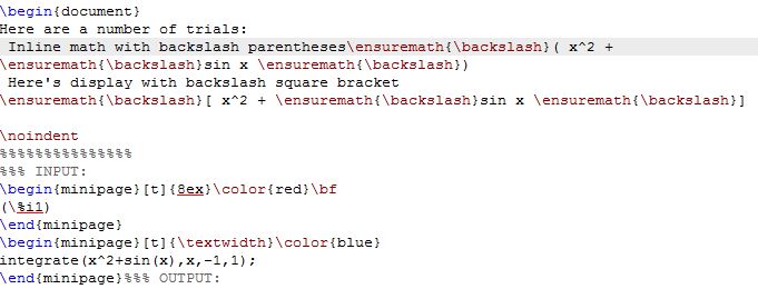
First, my wxMaxima document, with text cells that contain math formulas is shown in this screenshot:

maximaconsolecapture

After export to .tex , I get a file that includes the following latex source snippet.  Notice where I’d like inline math, there is in every case \ensuremath{\backslash}.

texsourcecapture

What is \ensuremath{\backslash} and why does wxMaxima insist on it?

I don’t have an answer for what or why, but it turns out all those \ensuremath{\backslash} statements don’t compile in pdfLaTeX.  A lot of error messages emanate from pdfLaTeX.  The resulting pdf is given below.  Notice the \( isn’t recognized as the start of LaTeX inline math.  The compiler gets the hint about math mode when it sees the superscript, but the \ensuremath{\backslash} gets in the way again and again:

maximapdfcapture

Yuck!  And all I really wanted in that latex source was \(  and \)…

Find and Replace All

I edited the .tex source with a find-replace-all every occurrence of \ensuremath{\backslash} with \    and the result is much nicer:

pdftextmathsnippet

However, there are still a bunch of pdflatex errors from the lines corresponding to the maxima input and output. Turns out anything that LaTeX finds in the maxima that wants to be in math mode, in this case the superscript x^2, results in an “inserted missing $”, kind of error.  Lots of them, in fact.

You can see that in the blue text in the graphic above:  the first occurrence of the variable x is not in math mode, then everything after the ^ is, which then makes the sin(x) appear incorrectly because latex would have wanted \sin, which wouldn’t make sense as a Maxima command.

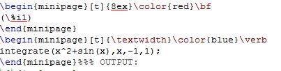
Maxima input looks better verbatim

To remedy the compiler errors and, in my opinion, make the maxima input clearer for the reader than it would have been if the LaTeX would have somehow known what to make of it, I further edited the latex code, inserting the LaTeX “verbatim” command \verb in each occurrence of maxima input:

texsourcecaptureverbatim

And the resulting pdfLaTeX compiled pdf looks great:

pdfgoodcapture

A surface, a tangent plane, a normal line

I set out to do a visualization that is basic to the multivariable calculus classroom:  plot a surface, a tangent plane, and a normal line.  I didn’t do it on the first try…or the second.

I had to learn some things about the draw3d functionality in Maxima and wxMaxima.  Here’s a great resource by Wilhelm Haager.  In the end I’m delighted at the amazing flexibility of that command, but still scratching my head a little about how this would appear to an otherwise uninitiated beginner to Maxima.

Here’s the html export of my session.

Multivariable Optimization in Maxima

I’ve been working on a few problems from multivariable calculus, with and without the method of Lagrange multipliers.  I’ve learned a lot about the solve command, and also become much more comfortable with the amazingly flexible plotting command wxdraw3d. The calling sequence of wxdraw3d looks a little daunting compared to wxplot3d, but the added flexibility — especially the ability to superimpose several plots on the same set of 3D axes — is really brilliant!

Here is the HTML export from my wxMaxima session.  You can get to the .wxmx file from a link at the bottom of that page.

Two Maxima Functions for Riemann Sums

Two early attempts at programming Maxima functions.  I’d love to hear your comments about how to make these work better.  Many thanks to the online community from whom I learned how to get this far!

The script is given at the bottom of this post.  Copy and paste into a file (in your working directory) called Riemann.mac, and then load into Maxima using

load(“Riemann.mac”);

Riemann

/* Two Maxima functions for introductory integral calculus
(c) 2016, themaximalist.org  */

/* RiemannSum
fn is the function to be integrated on the interval [a,b]
n rectangles
opt specifies:
0: left endpoints
1: midpoints
2: right endpoints
*/

RiemannSum(fn,a,b,n,opt):=
block([xx,s],
xx(i,n):= a+(i+opt/2)*(b-a)/n,
s: sum(ev(fn,x=xx(i,n)),i,0,n-1)*(b-a)/n,
float(s)

)$

/* RiemannRectangles to Draw rectangles
fn is the function to be integrated:
on the interval [a,b]
n rectangles
opt specifies:
0: left endpoints
1: midpoints
2: right endpoints
*/

load(draw)%

RiemannRectangles(fn,a,b,n,opt):=
block([xi,xx,rects,wxd],
xi(i,n):= a+i*(b-a)/n,
xx(i,n):= a+(i+opt/2)*(b-a)/n,
rects(n):=makelist(rectangle([xi(k,n),0], [xi(k+1,n),ev(fn,x=xx(k,n))]),k,0,n-1),
wxd(n):=apply(wxdraw2d,
append([xrange=[a-(b-a)/4, b+(b-a)/4],color=blue],
rects(n),
[transparent=true, explicit(fn,x,a, b)]
)
),
wxd(n)
)$


Root of a nonlinear equation, as the last step of an ODE solution

What better use for a computer algebra system than a problem whose solution you know intuitively, and for which the paper-and-pencil work feels too daunting to start?  Here’s a problem that exploits what we know about the solutions of damped driven oscillators, making use of the usual ODE capabilities in Maxima, together with a nonlinear solve with find-root at the end.

Limits for functions of two variables

The Maxima limit command is limited (ha ha) to functions of a single variable.  We can use Maxima to approach the issue just as we do by hand computation:  reduce to single variable limits by considering that the vector variable (x,y) approaches the limit point (a,b) along paths of the form (x, y(x)).  Here’s a nice example from my Multivariable Calculus Class