In an earlier post I detailed the Maxima functions contained the MATH214 package for use in my multivariable calculus class. The package at that link has now been updated with some further integration utilities: integrate2() and integrate3() for double and triple integrals and integrateSurf() for surface integrals of vector fields in 3D. I’ve posted examples with applications to Green’s Theorem and Gauss’s Theorem.
Here’s a test drive of the surface integration function using a Stokes theorem example I found on the web:
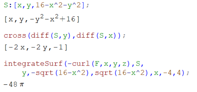
Verify Stokes theorem for the surface S described by the paraboloid z=16-x^2-y^2 for z>=0
and the vector field
F =3yi+4zj-6xk
First the path integral of the vector field around the circular boundary of the surface using integratePathv3() from the MATH214 package

And also the surface integral using integrateSurf(). Notice that in the order of integration we specify in integrateSurf(), (first y then x) the surface normal vector computed with cross() in that same variable order points inward—the negative orientation. We reverse the direction with an extra negative inside the surface integral.
Although they are included in the MATH214 package, here are the functions used above:
integrateSurf(F,S,uu,aa,bb,vv,cc,dd):=block(
 [F2],
 F2:psubst([x=S[1],y=S[2],z=S[3]],F),
 integrate(integrate(trigsimp(F2.cross(diff(S,uu),diff(S,vv))),uu,aa,bb),vv,cc,dd));

cross(_u,_v):=[_u[2]*_v[3]-_u[3]*_v[2],_u[3]*_v[1]-_u[1]*_v[3],_u[1]*_v[2]-_u[2]*_v[1]]$

curl(f,x,y,z):=[ diff(f[3],y)-diff(f[2],z),curl(f,x,y,z):=[ diff(f[3],y)-diff(f[2],z),                     diff(f[1],z)-diff(f[3],x),   diff(f[2],x)-diff(f[1],y) ]$
integratePathv3(H,r,t,a,b):=block(
[H3],
H3:psubst([x=r[1],y=r[2],z=r[3]],H),
 integrate( trigsimp(H3.diff(r,t)),t,a,b)
);


 ,
,  ,
, ) in one step to use the antiderivative
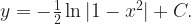

 , but still…
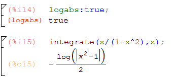
 ,
,