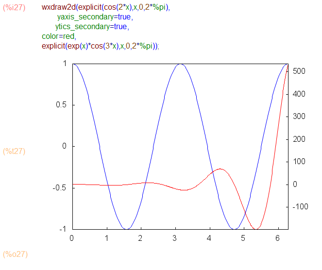
In MATLAB, I occasionally have need for the plotyy() command for making a plot of two different functions with widely varying scales.
Turns out Maxima draw has an equivalent functionality by setting the option yaxis_secondary:

In MATLAB, I occasionally have need for the plotyy() command for making a plot of two different functions with widely varying scales.
Turns out Maxima draw has an equivalent functionality by setting the option yaxis_secondary:
pause([options]):=block([tsecs],
    tsecs:assoc('pausetime,options,0),
    if tsecs=0 then
       read("Execution Paused...enter any character then CTRL-ENTER")
    else(
        disp(sconcat("paused for ", tsecs," seconds")),
       ?sleep(tsecs)),
    return("")
);
In MATLAB, I often use the subplot() command to make an array of multiple plots in a single figure.
In Maxima, we can achieve that by generating each of the subplots using gr2d(), and then putting them all together with a call to draw() or wxdraw():

There’s an optional columns argument — the subplots are drawn row-wise in an array with the specified number of columns:
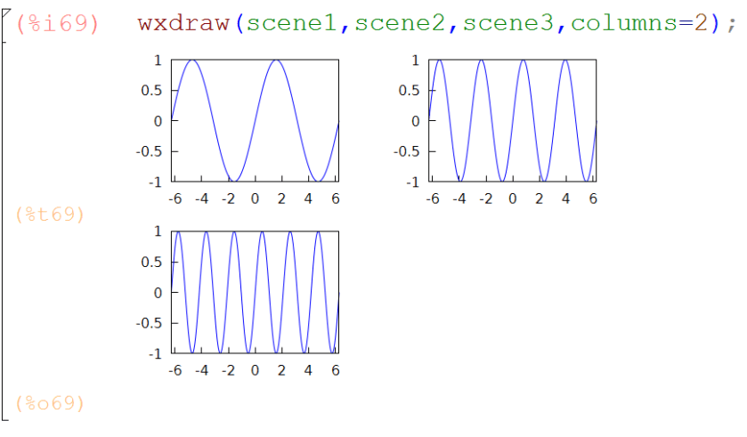
And of course all this works for 3d plots using gr3d():

In Matlab and RStudio, I love the ability to recall a command I’ve already typed using the up arrow key. Today I discovered alt up arrow to do the same in wxMaxima!
This is really the best implementation of function templates I’ve seen in an IDE:
In wxMaxima, if I type inte and then ctrl shift k, I see a popup menu of possible completions. Choosing integrate results in an input cell template that looks like:
integrate(<expr>,<x>)
Pressing Tab highlights <expr> and I simply type the expression to be integrated. A second press of Tab key highlights <x> and I type the name of the independent variable.
But wait, there’s more: this works for any currently defined function—including user defined functions.
**UPDATE** In the newer versions of wxMaxima (since v15.10) Ctrl+Tab and Shift+Ctrl+Tab also trigger autocompletion.

Notepad++ is lots of people’s favorite text editor for Windows. I use it every day.
A little googling around led me to a Notepad++ user-defined syntax highlighting file for the Maxima language, written by David Scherfgen and shared at the Maxima-Discuss list.
I made a little change to the file that overcame a nagging difficulty — I found that .mac file extensions weren’t automatically being recognized upon opening.
Here’s a link to my modifed file.
To include Maxima syntax highlighting in Notepad++ do this:
I was looking recently at the PYPL PopularitY of Programming Language.
That site ranks popularity of programming languages (Java is #1) using Google Trends tools based on searches of the form <Language Name> Tutorial. I did my own Google Trend search, comparing the 3M of Computer Algebra Systems: Maple, Mathematica, and Maxima using the Tutorial criteria as at PYPL.
With the data from Google Trends, I computed the proportion of the total 3M monthly searches for each program. Here’s how that looks over time since 2004:

It appears to me that Maxima is slowly and steadily gaining with nearly 20% share, Maple is currently at about 30%, and Mathematica at 50%. Does anybody know what happened between 2006 and 2013 to account for the increase in popularity of Mathematica and decrease for Maple?
I’ve put together a collection of functions — some direct quotes of other contributed functions, some renamed or repackaged, and some newly implemented — for various needed tasks in my undergraduate ordinary differential equations course.
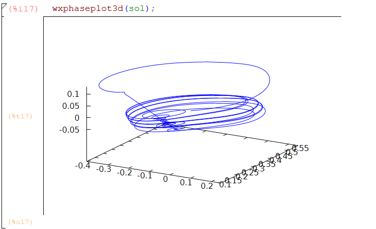
I’ve written elsewhere about the Backward Difference Formula implementations, the phase space visualization functions, the matrix extractors, and the numerical solutions plotters.
The package includes my home-grown help utility.
You can download the package MATH280.mac
…and if you’re interested, here’s my multivariable calculus package MATH214.mac
MATH280.mac contains:
 wxphaseplot2d(s)
 wxphaseplot3d(s)
 phaseplot3d(s)
 wxtimeplot(s)
 plotdf(rhs)
 wxdrawdf(rhs)
 sol_points(numsol,nth,mth)
 rkf45(oderhs,yvar,y0,t_interval)
 BDF2(oderhs,yvar,y0,t_interval)
 BDF2a(oderhs,yvar,y0,t_interval)
 odesolve(eqn,depvar,indvar)
 ic1(sol,xeqn,yeqn)
 ic2(sol,xeqn,yeqn,dyeqn)
 eigU(z)
 eigdiag(z)
 clear()
 -
 -
 for any of the above functions,
 help(function_name) returns help lines for function_name
 -
 Last Modified 5:00 PM 3/27/2017
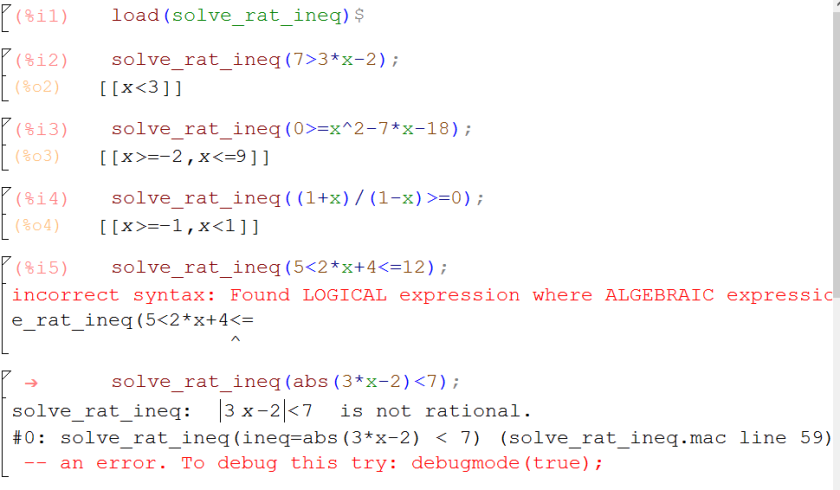
There is an undocumented user-contributed feature of Maxima for rational inequalities: solve_rat_ineq().
Here are few examples of its capabilities and limitations:
Yesterday I needed a cumulative sum function in Maxima to do the job of cumsum() in R and MATLAB, but couldn’t find anything. So here’s a one-liner that does the trick for a list:
cumsum(L):=makelist(sum(L[i],i,1,n),n,1,length(L))$

Maxima comes with a few well-implemented numerical ODE solvers — rk() and rkf45() — and I’ve written in a previous post about my variable stepsize implementation of the 2nd order backward differentiaion formula for stiff systems BDF2a().
Plotting the resulting numerical solutions — which is a list of lists of the form
[[indvar, depvar1, depvar2,… ], [indvar, depvar1, depvar2,… ], … ]
with each of the sublists representing the state of the system at a discrete time — requires a little familiarity with list functions like makelist() and map().
Here are a few little helper routines to make that quicker:
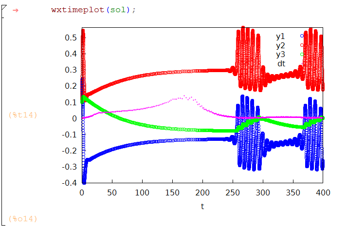
This is mainly a teaching tool for my ordinary differential equations course, taking the output of the solver and, assuming there aren’t more than three dependent variables, plotting all the dependent variables vs the independent variable on the same set of axes, with a representation of the step size.
I wrote about these in another post
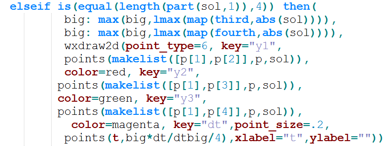
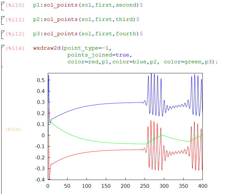
This is a more general purpose function. Given the output of the numerical ode solver, this constructs a points() subcommand ready to plug into draw2d(). This allows for the full generality of draw2d: colors, axis labels, point points,
Especially useful for plotting results from more than one call to the solver, such as when we need to see the effect of changing a parameter value:
Below I’ve pasted the code for the plots, and also for the interesting differential equations from Larter et al in Chaos, V.9 n.3 (1999)
(tw:(cosh((Vi-V3)/(2*V4))^(-1)),
m:(1/2)*(1+tanh((Vi-V1)/V2)),
w:(1/2)*(1+tanh((Vi-V3)/V4)),
aexe:aexe1*(1+tanh(Vi-V5)/V6),
ainh:ainh1*(1+tanh((Zi-V7)/V6))
)$

(rhs1:-gCa*m*(Vi-1)-gK*Wi*(Vi-ViK)-gL*(Vi-VL)+I-ainh*Zi,
 rhs2:(phi*(w-Wi)/tw),
 rhs3:b*(c*I+aexe*Vi)
 )$

(V1:-.01,V2:0.15,V3:0,V4:.3,V5:0,V6:.6,V7:0,
 gCa:1.1,gK:2,gL:0.5,VL:-.5,ViK:-.783,phi:.7,tw:1,
 b:0.0809,c:0.22,I:0.316,aexe1:0.6899,ainh1:0.695)$

 load(rkf45);

 sol:rkf45([''rhs1,''rhs2,''rhs3],[Vi,Wi,Zi],[.1,.1,.1],[t,0,400],
             report=true,absolute_tolerance=1e-8)$
sol_points(numsol,nth,mth):=points(map(nth,numsol),map(mth,numsol));
/* wxtimeplot takes the output of sol: rk45 and plots
 up to 3 dependent variables
plus the scaled integration step size vs time*/
wxtimeplot(sol):=block(
[t0,t,tt,dt,big,dtbig],
t0:map(first,sol),
t:part(t0,allbut(1)),
tt:part(t0,allbut(length(t0))),
dt:t-tt,
dtbig:lmax(dt),
big:lmax(map(second,abs(sol))),
if is(equal(length(part(sol,1)),3)) then(
 big: max(big,lmax(map(third,abs(sol)))),
 wxdraw2d(point_type=6, key="y1",
 points(makelist([p[1],p[2]],p,sol)),
 color=red, key="y2",
 points(makelist([p[1],p[3]],p,sol)),
 color=magenta, key="dt",point_size=.2,
 points(t,big*dt/dtbig/4),xlabel="t",ylabel=""))
elseif is(equal(length(part(sol,1)),2)) then
 wxdraw2d(point_type=6, key="y1",
 points(makelist([p[1],p[2]],p,sol)),
 color=magenta, key="dt",point_size=.2,
 points(t,big*dt/dtbig/4),xlabel="t",ylabel="")
elseif is(equal(length(part(sol,1)),4)) then(
 big: max(big,lmax(map(third,abs(sol)))),
 big: max(big,lmax(map(fourth,abs(sol)))),
 wxdraw2d(point_type=6, key="y1",
 points(makelist([p[1],p[2]],p,sol)),
 color=red, key="y2",
 points(makelist([p[1],p[3]],p,sol)),
 color=green, key="y3",
 points(makelist([p[1],p[4]],p,sol)),
 color=magenta, key="dt",point_size=.2,
 points(t,big*dt/dtbig/4),xlabel="t",ylabel=""))
 );