Partial Fraction Decomposition Using Complex Factors

A few days ago I wrote about my solution for factoring a polynomial into factors corresponding to complex roots,  factorC.

One of the uses for that utility is to perform a partial fractions decomposition of rational functions.  Here’s a complex partial fraction function that uses factorC and the built-in Maxima function partfrac.

partfracC

partfracC(_f,_z):=block(
[d,fd],
d:denom(_f),
fd:factorC(d,_z),
partfrac(1/fd,_z)
);

Complex Factors of Real and Complex Polynomials

I’m getting ready for my fall Complex Variables class.  I noticed that the built-in Maxima function residue doesn’t reliably do the right thing.  My goal is to make some improvements to  Maxima residue calculations in Maxima over the course of the next month.

As I started to look at some test cases, I realized I didn’t know how to factor a polynomial into complex factors.  In the simplest case:

realfactor

but I wanted to see

manual_complexfactor

Maybe someone will find this and let me know that there’s a simple way to make that happen using existing Maxima commands.  Until then, I’ve written a little utility  to identify the roots (both real and complex) of a polynomial and return a factorization.  Here’s an example, and the code.  Notice that it only works as well as the root finder solve.  I tried to upgrade to the more robust to_poly_solve,  but I don’t yet know how to handle multiplicities in that case.

factorCexample

factorC(_f,_z):=block(
[s,n,m,fp,j],
fp:1,
/* This commented code was meant to use the
more robust solver to_poly_solve, but 
I couldn't understand how to handle multiplicities
ss:args(to_poly_solve(_f,_z)),
s:create_list(ss[k][1],k,1,length(ss)),*/
s:solve(_f,_z),
m:multiplicities,
n:length(s),
for j:1 thru n do 
 if lhs(s[j])#0 
 then fp:fp*(_z-(rhs(s[j])))^m[j],
 fp:fp*divide(_f,fp)[1],
fp
);

Computing and Visualizing Path Integrals of Vector Fields

A few months ago, I posted my path integral functions, which are included in the MATH214 package.  Recently, I came across something I’d been looking for:  a Maxima utility for visualizing vector fields.  Its in the Maxima/Share directory under drawutils.

Written in 2010 by Donald J Bindner, the commands plot_vector_field and plot_vector_field3d do almost everything I was looking for.  The drawback is that I wanted to plot the vector fields along with the integration path.  I modified those two commands slightly into versions called make_vector_field  and make_vector_field3d to produce the lists of vectors for plugging into draw2d and draw3d, so that I could include the vector fields in  bigger graphics calls.  My modifications are available here.  The package includes my home-baked help utility.

Here’s what the path integral command and the vector field generator look like on an example from chapter 13 of Stewart’s “Calculus Concepts and Contexts”

StewartPathIntegralExample

StewartVectorFieldIntegralPicture

Solvers!

A few months ago, when I was very new to Maxima, I posted my solutions to several multivariable optimization problems, and included a standard constrained optimization example for which the built in command solve failed.

Here’s the problem:

MinVolConstArea

In my multivariable calculus class, we’ve just encountered that problem again.  What my students and I discovered was that the order of the variables as specified by the user in the argument list caused the command to either succeed or fail, as you can see from the first two lines below:

Ksolve

I wrote to the experts at maxima-discuss@lists.sourceforge.net.  They replied en masse very quickly and were very generous with their time and advice. They verified the problem, pointing out that solving systems of equations is really complicated, and that the solve program seeks to solve for the variables one at a time and things can go wrong if an inauspicious order of variables is followed.

The experts also tried our problem with the package to_poly_solve, and happily it succeeded without the hassle of needing to specify the variables in the right order.  For solve users who reference the solutions it produces as elements of a list, direct use of to_poly_solve presents a  challenge due to output in a format different from that of solve  — t0_poly_solve returns solutions as a set with %union.

I’ve written a little wrapper Ksolve.mac that is called like solve as illustrated above.

In Ksolve if an initial call to solve fails, the process automatically upgrades to to_poly_solve in several variations, and  (hopefully) returns solutions in the same format as solve.


Maxima for maxima (and minima) of functions z=f(x,y)


surfacecontours

Together with the 3D graphing capabilities of Maxima, we can bring  symbolic differentiation and the numerical solver to bear when we seek local extrema of a surface.

Here is a link to the html export of a wxMaxima session where I work on two examples from my multivariable calculus class.  And here is the wxMaxima session.

:=, ”(), define and div, grad, curl

I recently posted about : and :=  for defining functional expressions.  I’m starting to enjoy these emoji-like constructions 😉

This is another  colon-equals post.  This time for defining functions involving the maxima differentiation command diff.

Notice below that if we define a function with :=, the naive use of :=diff doesn’t produce a derivative with the expected results upon evaluation.

colonequaldiff

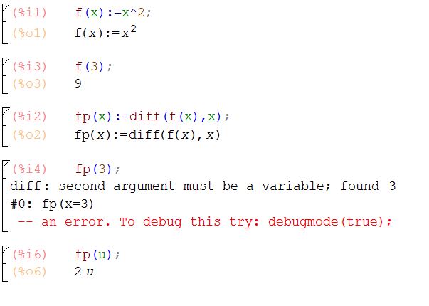
In fact, it’s a good thing that :=diff works like that.  The error with fp(3) above comes from the fact that we’ve actually defined an operator that differentiates the function with respect to the argument we pass…in the case above, differentiating with respect to the symbol u makes sense, while differentiating with respect to the constant 3 doesn’t.

So how to make the derivative function do what we want?  Two ways, that are subtly different, in ways I’m not completely sure of.  More about that when I learn more :-).
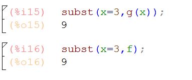
First is define,

definediff

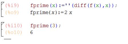
Also you can use    ”()       quote-quote with parens around the whole right hand side:

quotequotediff

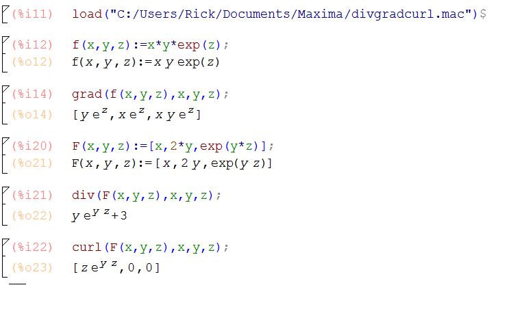
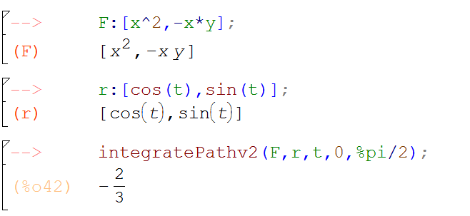
I used define to write functions for vector valued 3D curves in an earlier post.   In figuring this out, I also learned that the :=diff form is really useful.  Below are three little functions in which I use :=diff to define the vector calculus operators grad, div and curl.  Notice that we pass the function f as an argument, and the :=diff form allows Maxima to differentiate them behind the scenes and return the results of the grad, div, and curl operators as you’d expect. These versions of div, grad and curl behave differently, and for me more as expected, than the functions of those names included in the Maxima vect package.  You can download the .mac file here.

/* Three Maxima functions for the multivariable calculus operators  grad, div, and curl
TheMaximaList.org, 2016
*/

grad(f,x,y,z):=[diff(f,x),diff(f,y),diff(f,z)]$

div(f,x,y,z):=diff(f[1],x)+diff(f[2],y)+diff(f[3],z)$

curl(f,x,y,z):=[ diff(f[3],y)-diff(f[2],z),
diff(f[1],z)-diff(f[3],x),
diff(f[2],x)-diff(f[1],y) ]$

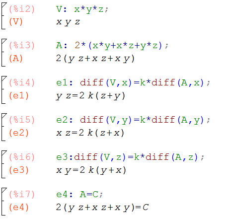
Here is a screenshot showing how to call these functions:

divgradcurl

$latex \int x^2 dx$

I’m testing the latex math-mode utility in WordPress.com.  The first thing to know is that based on the way the title of this post appears, the latex utility doesn’t work in post titles.

The rub here is that MathJax would be the natural solution, but WordPress.com isn’t compatible with JavaScript.  

That leaves us with $, followed by the word latex, followed by my latex markup, followed by a closing $ , which I illustrate  below with a screenshot because I don’t know how to quote a string verbatim in WordPress:

preform

This works OK as inline style math \int x^2 dx and I think we could simulate display math mode like this with manual paragraph centering and with the optional size argument &s=1 inside the dollar signs (the default size is 0)

\int x^2 dx

and then back to inline for f(x).

And there it is.

The official guide to the  WordPress \LaTeX utility  can be found here.

Functions, :, and :=

I’m really posting this for myself to act as a big paperweight.  Whenever I forget about :=  and : for functions in Maxima, I can refer to this page.

The gist:

  • g(x):=x^2  results in a function you can evaluate as g(3)
  • f: x^2 results in an expression you can evaluate with ev(f,x=3)
  • ev works with both:  ev(g(x),x=3)  or ev(f,x=3)
  • also subst(x=3,f) and subst(x=3,g(x))
  • based on our definition, g doesn’t have a meaning…only  g(x) does
  • likewise, f(3) doesn’t have a meaning here…only the symbol f does
  • finally h:=x^2 gives an error — explicit dependent variable needed with :=

colonequals

subst

colonequalserror