Solve Ax=b in Maxima, part 2

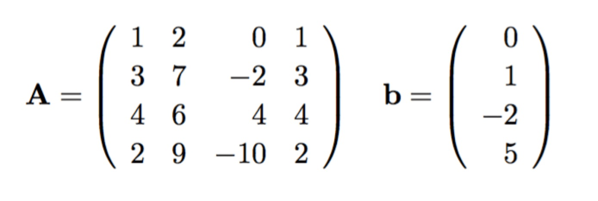
In a previous post, I included my little coding project to implement a general backsolve() function to use with the built-in maxima matrix function echelon(), producing an easy-to-call matrix solver matsolve(A,b).  The result is meant to solve a general matrix vector equation Ax=b , including cases when A is non-square and/or non-invertible.

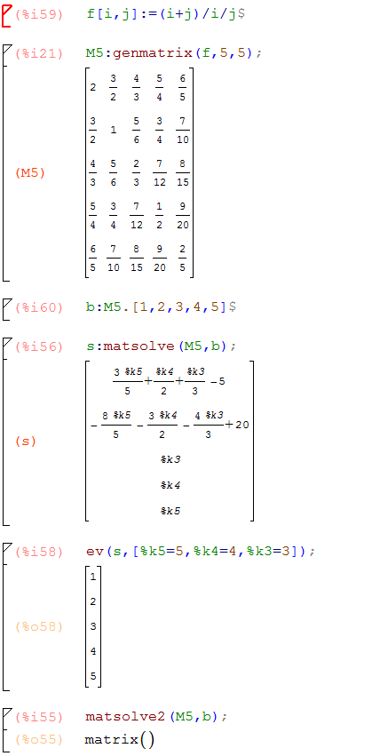
Here’s a quicker approach — convert the matrix into an explicit system of equations using a vector of dummy variables, feed the result into the built-in Maxima function linsolve(), and then extract the right hand sides of the resulting solutions and put them into a column vector.

The two methods often behave identically, but here’s an example that breaks the linsolve() method, where the backsolve() method gives a correct solution:

matsolve2breaks


*Note, I’ve found that the symbol rhs is a very popular thing for users to call their problem-specific vectors or functions.  Maxima’s  “all symbols are global” bug/feature generally wouldn’t cause a problem with a function call to rhs(), but the function map(rhs, list of equations)  ignores that rhs() is a function and uses user-defined rhs.  For that reason I protect that name in the block declarations so that rhs() works as expected in the map() line at the bottom.  I think I could have done the same thing with a quote: map(‘rhs, list of equations).

matsolve2(A,b):=block(
 [rhs,inp,sol,Ax,m,n,vars],
 [m,n]:[length(A),length(transpose(A))],
 vars:makelist(xx[i],i,1,n,1),
 Ax:A.vars,
 inp:makelist(part(Ax,i,1)=b[i],i,1,n,1),
 sol:linsolve(inp,vars),
 expand(transpose(matrix(map(rhs,sol))))
);
Advertisement

A Little Maxima Function to Find the Dimensions of a Matrix

**Update**  I didn’t find it it in documentation for quite a while, but there is a built-in Maxima function matrix_size()  in the package linearalgebra that does what this little one-liner does**

linearalgebrapackage

I really wanted a Maxima function that works something like MATLAB size() to easily determine the number of rows and columns for a matrix M.  
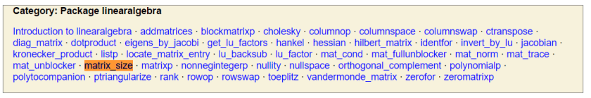
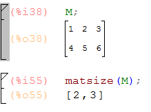
In Maxima, length(M) gives the number of rows, and so length(transpose(M)) gives the number of columns.  I put those together in a little widget matsize() that returns the list [m,n] for an m \times n matrix M:

matsize

matsize(A):=[length(A),length(transpose(A))];

Extracting Matrices from the Output of eigenvectors()

In class I sometimes need to use matrices of eigenvalues and eigenvectors, but the output of eigenvectors() isn’t particularly helpful for that out of the box.

Here are two one-liners that work in the case of simple eigenvalues.  I’ll post updates as needed:

First eigU(), takes the output of eigenvectors() and returns matrix of eigenvectors:

eigU(v):=transpose(apply('matrix,makelist(part(v,2,i,1),i,1,length(part(v,2)),1)));

And eigdiag(), which takes the output of eigenvectors() and returns diagonal matrix of eigenvalues:

eigdiag(v):=apply('diag_matrix,part(v,1,1));

eigs

For a matrix with a full set of eigenvectors but eigenvalues of multiplicity greater than one, the lines above fail.  A version of the above that works correctly in that case could look like:

eigdiag(v):=apply('diag_matrix,flatten(makelist(makelist(part(v,1,1,j),i,1,part(v,1,2,j)),j,1,length(part(v,1,1)))));

eigU(v):=transpose(apply('matrix,makelist(makelist(flatten(part(v,2))[i],i,lsum(i,i,part(v,1,2))*j+1,lsum(i,i,part(v,1,2))*j+lsum(i,i,part(v,1,2))),j,0,lsum(i,i,part(v,1,2))-1)));

Using Maxima To Do Some Math Described in the Movie “Hidden Figures”

I looked in the NASA archives for the work of Katherine Johnson described so dramatically in the film “Hidden Figures”.  I found this 1960 paper:

nasa_title

In particular, I was struck by the film’s use of “Euler’s Method” as the critical plot point, and sadly couldn’t find anything about the use of that method in the archive, nor mention of it in the text of  Margot Lee Shetterly’s book on which the film “Hidden Figures” is based.

I did however read in the paper about an “iterative procedure” needed to solve for one variable.

Turns out the sequence of equations described in the report, when assembled into an expression in the single variable of interest, defines  a contraction mapping and so converges by functional iteration, as is numerically demonstrated in the paper.

At the bottom I’ve linked a fuller treatment in a .wxmx file.  Briefly, the authors describe the problem:

nasaeq19

nasaeq20

nasaeq89

nasa_iteration

Here’s everything from the paper needed to do that in Maxima:

nasaconstants1

nasaconstants2

nasaconstants3

I put together equations 19,20,8, and 9, together with all those constants defined by the paper and customized trig function that act on angles measured in degrees, into an expression of the form

  \theta_{2e}=F(\theta_{2e})

and applied the built-in Maxima numerical solver find_root().  The result agrees reasonably well with the result  \theta_{2e}=50.806 
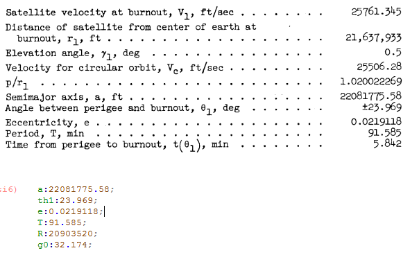
quoted in the paper.

nasaiteration_findroots

In the above, I computed the derivative of the mapping F 
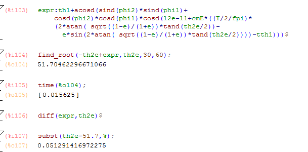
evaluated at the solution and found that the value is much less than one, showing it is a contraction.

Here’s my full wxMaxima session.

trigexpand(), trigsimp() and an oscillatory solution of a 2nd order linear differential equation

I was working on a differential equations homework problem and it took me a few tries to remember how to simplify a trig expression.  So, I thought I’d put the results here to remind myself and others about trigexpand().

The second order linear equation is

 y''+y'+y=0 \;\;\;\;\;\; y(0)=1, y'(0)=0

odesol

Now I asked my students to use the identities

  A= \sqrt{C_1^2 + C_2^2}  and  \tan \phi=C_2/C_1

to write the equation equivalently as

 y=A e^{-x/2} \cos \left( \frac{\sqrt{3}}{2}  x -\phi \right)

odeoscillparams

Finally, I wanted to use Maxima to show these two expressions are equivalent.  I reflexively used trigsimp() on the difference between the two expression   (the name says it all, am I right?)  but the result was complicated in a way that I couldn’t recover…certainly not zero as I hoped.  A few minutes of thought and I remembered trigexpand() which, followed by a call to trigsimp(), gives the proof:

odetrigexpand

Complex roots of unity and the map() function

Here’s a little application from Complex Variables class that uses map() to repeatedly apply Maxima functions to each element in a list.

We want to find the complex 6th roots of 1 — there should be six such complex numbers z 
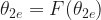
that solve the equation

  z^6=1

sixthrootseqn

Notice the solutions are returned as equations…this is sometimes really handy, but for now we want to isolate the right hand side of each equation. The command rhs(), when applied to an equation, returns just the right side. We can apply the rhs command to all the equations contained in our solution using the Maxima command map():

sixthrootsmap

Finally, with the real and imaginary parts extracted, we can plot the six roots

sixthrootsplot


An odd gnuplot error and a work-around using maxima_tempdir

***Update***********************

I also have this problem in the latest windows installation—on the same machine that long filenames were never a problem before in Maxima.  To fix it choose the sbcl version of maxima, as described at My Windows Installation.

*********************************

I have a student running wxMaxima on his windows laptop.  He has partitioned his hard drive so he can run Windows 10 as well as other operating systems.

When he attempts any plotting command, he gets an error:

gnuplot_error

The part of the error message with directory name TANUSH~1 says to me that there is some problem with the long directory name, possibly also a problem caused by a space in that directory name, possibly due to the way those new partitions are formatted.

As a workaround, we set the maxima option maxima_tempdir to point to another directory and all worked as expected:

maxima_tempdir

Of course, that new directory will now fill up with files with names like maxout_xxxx.dat and maxout_xxxx.gnuplot, but that was already happening in the default directory.  A natural feature for wxMaxima to include in future releases would be to clean up the directory by deleting all those files when the program is stopped…

3D Printing and Maxima

In response to several nearly simultaneous queries, I’ve been working this week on generating a 3D  plot  and creating a mesh file from within Maxima  that is suitable for exporting to a 3D printer.

As a guide, I used this 2012 article from the Mathematical Intelligencer by Henry Segerman.  The idea is to draw a surface using traces made from parametric tubes, then export that to a .PLY format file.

Here’s my prototype for the process of generating the surface, reading in the resulting gnuplot data file, identifying faces appropriately, and writing into a .PLY file.

That isn’t yet ready for the 3D printer, but I could load it into the free program MeshLab, and from there convert to .STL

Here’s my figure from Maxima:

pringle

And the resulting .PLY file loaded into MeshLab


saddle_meshdraw

Here’s a few seconds of video from the printing process

And 2.5 hours later, the low resolution first-try 3D printed object:

3dprintverision01

Visualizing Complex Functions by their images over concentric circles

A few weeks ago I posted my Maxima code for visualizing complex function by their images over a grid of line segments in the complex plane.  Here are a few images from an experiment of plotting the image of complex function over concentric circles, centered at the origin, traversed in the counterclockwise direction.  The first image below shows the identity map.  The colors are in ROYGBIV rainbow order, as noted in the legend, which gives the radius of the pre-image circles.  The second image is for the function f(z)=(z-1/2)(z-1).  Notice for the smallest radius pre-image, the image under f is largely unchanged.  As radius grows the image forms a loop then doubles on itself.  Here’s a fun insight:  that looping behavior occurs at radius .75, a circle containing a point z at which f'(z)=0.  More on this later, but its exciting to find a geometric significance of a zero of the derivative, considering how much importance such points have in real calculus.  Finally the third figure shows really interesting behavior for the function f(z)=\frac{1}{(z-1/2)(z-1)}.  Notice again the looping brought about by points at which the derivative is zero.  Notice also the change in direction of the image each time we cross over a pole—that is a root of the denominator.  The maxima code is given below.

/* wxdrawcircleC
 plot the traces of complex valued function _f
 along concentric circles |z|=r for 0<r <=1
 blue - images of _f along horizontal lines
 red - images of _f along vertical lines */
wxdrawcircleC(_f):=block(
[fx,fy,fxt,fyt,pl,j,ncirc,r,theta_shift,lm,l,dx,dy,dxy,v,nt],
ratprint:false,
fx:realpart(rectform(subst(z=x+%i*y,_f))),
fy:imagpart(rectform(subst(z=x+%i*y,_f))),
pl:[],
nt:200,
r:2,
ncirc:7,
theta_shift:%pi/20,
/* get the max modulus for computing length of arrows */
lm:0,
for n:1 thru ncirc do (
l:cons(lm,makelist(cabs(subst(z=r*n/7*exp(%i*t),_f)),t,0,2*%pi,.5)),
 lm:lmax(l)
 ),
 for j:1 thru ncirc do(
 /*first the images of the circles */
 fxt:subst([x=r*cos(t)*j/ncirc,y=r*sin(t)*j/ncirc],fx),
 fyt:subst([x=r*cos(t)*j/ncirc,y=r*sin(t)*j/ncirc],fy),
 pl:cons([parametric(fxt,fyt,t,0,2*%pi)] , pl),
 pl:cons([color=colorlist(j)],pl),
 pl:cons([key=string(r*j/ncirc)],pl),
 /* now the arrows */
 dx:subst(t=3/nt,fxt)-subst(t=0,fxt),
 dy:subst(t=3/nt,fyt)-subst(t=0,fyt),
 dxy:sqrt(dx^2+dy^2),
 v:vector([subst(t=0,fxt),subst(t=0,fyt)],[lm*dx/dxy/20,lm*dy/dxy/20]),
 pl:cons([v],pl),
 pl:cons([head_length=lm,head_angle=1],pl),
 pl:cons([color=colorlist(j)],pl),
 pl:cons([key=""],pl)
 ),
pl:cons([xlabel="",ylabel=""],pl),
pl:cons([nticks=nt],pl),
pl:cons([grid=on],pl),
apply(wxdraw2d,pl)
);

Visualizing Complex Functions with Conformal Mapping

For the thoroughly modern calculus student, an introduction to Complex Variables is all the more daunting because we don’t have the kind of geometric intuition-building machinery available to us for functions f: C \rightarrow C as we did for real-valued functions in calculus.  Not that attempts haven’t been made….  In the coming weeks, I want to work on several techniques in Maxima.  Here’s a first approach:  conformal maps.  The code drawgridC below is limited in its versatility, but couldn’t be simpler to call.  Here are some examples,

/* plot the traces of complex valued function _f
 along grid lines in the square
 -1 <= Real(z) <= 1, -1<=Ima(z)<=1
 blue - images of _f along horizontal lines
 red - images of _f along vertical lines */
drawgridC(_f):=block(
[fx,fy,fxt,fyt,pl,j,ngrid],
fx:realpart(rectform(subst(z=x+%i*y,_f))),
fy:imagpart(rectform(subst(z=x+%i*y,_f))),
pl:[],
ngrid:19,
 for j:0 thru ngrid do(
 fxt:subst([x=-1+j*2/ngrid,y=t],fx),
 fyt:subst([x=-1+j*2/ngrid,y=t],fy),
 pl:cons([parametric(fxt,fyt,t,-1,1)] , pl)
 ),
pl:cons([color=red],pl),
 for j:0 thru ngrid do(
 fxt:subst([y=-1+j*2/ngrid,x=t],fx),
 fyt:subst([y=-1+j*2/ngrid,x=t],fy),
 pl:cons([parametric(fxt,fyt,t,-1,1)] , pl)
 ),
pl:cons([color=blue],pl),
pl:cons([xlabel="",ylabel=""],pl),
pl:cons([nticks=200],pl),
apply(wxdraw2d,pl)
);